Data transformations

Lecture 10

2025-04-10

Introduction to factors

Prerequisites

  • Base R provides some basic tools for creating and manipulating factors.
  • We’ll supplement these with the forcats package, which is part of the core tidyverse. It provides tools for dealing with categorical variables (and it’s an anagram of factors!) using a wide range of helpers for working with factors.
library(tidyverse)

Factors

Factor basics

Imagine that you have a variable that records month:

x1 <- c("Dec", "Apr", "Jan", "Mar")

Factor basics

Using a string to record this variable has two problems:

  1. There are only twelve possible months, and there’s nothing saving you from typos:

    x2 <- c("Dec", "Apr", "Jam", "Mar")
  2. It doesn’t sort in a useful way:

    sort(x1)
    [1] "Apr" "Dec" "Jan" "Mar"

Factor basics

You can fix both of these problems with a factor.

To create a factor you must start by creating a list of the valid levels:

month_levels <- c(
  "Jan", "Feb", "Mar", "Apr", "May", "Jun",
  "Jul", "Aug", "Sep", "Oct", "Nov", "Dec"
)

Factor basics

Now you can create a factor:

y1 <- factor(x1, levels = month_levels)
y1
[1] Dec Apr Jan Mar
Levels: Jan Feb Mar Apr May Jun Jul Aug Sep Oct Nov Dec
sort(y1)
[1] Jan Mar Apr Dec
Levels: Jan Feb Mar Apr May Jun Jul Aug Sep Oct Nov Dec

Factor NA

And any values not in the level will be silently converted to NA:

x2 <- c("Dec", "Apr", "Jam", "Mar")
y2 <- factor(x2, levels = month_levels)
y2
[1] Dec  Apr  <NA> Mar 
Levels: Jan Feb Mar Apr May Jun Jul Aug Sep Oct Nov Dec

Factor NA

This seems risky, so you might want to use forcats::fct() instead, which will throw a error warning:

y2 <- fct(x2, levels = month_levels)
Error in `fct()`:
! All values of `x` must appear in `levels` or `na`
ℹ Missing level: "Jam"

Factor sorting

Sorting alphabetically is slightly risky because not every computer will sort strings in the same way. So forcats::fct() orders by first appearance in the original vector:

fct(x1)
[1] Dec Apr Jan Mar
Levels: Dec Apr Jan Mar

Factor access

If you ever need to see the set of valid levels directly, you can do so with levels():

levels(y2)
 [1] "Jan" "Feb" "Mar" "Apr" "May" "Jun" "Jul" "Aug" "Sep" "Oct" "Nov" "Dec"

Reading factors from CSV

Factors in CSV files

You can also create a factor when reading your data with readr with col_factor():

csv <- "
month,value
Jan,12
Feb,56
Mar,12"

df <- read_csv(csv, col_types = cols(month = col_factor(month_levels)))
df$month
[1] Jan Feb Mar
Levels: Jan Feb Mar Apr May Jun Jul Aug Sep Oct Nov Dec

Factors reordering and releveling

Factor reorder

Imagine the following plot, what would you like to ameliorate it for
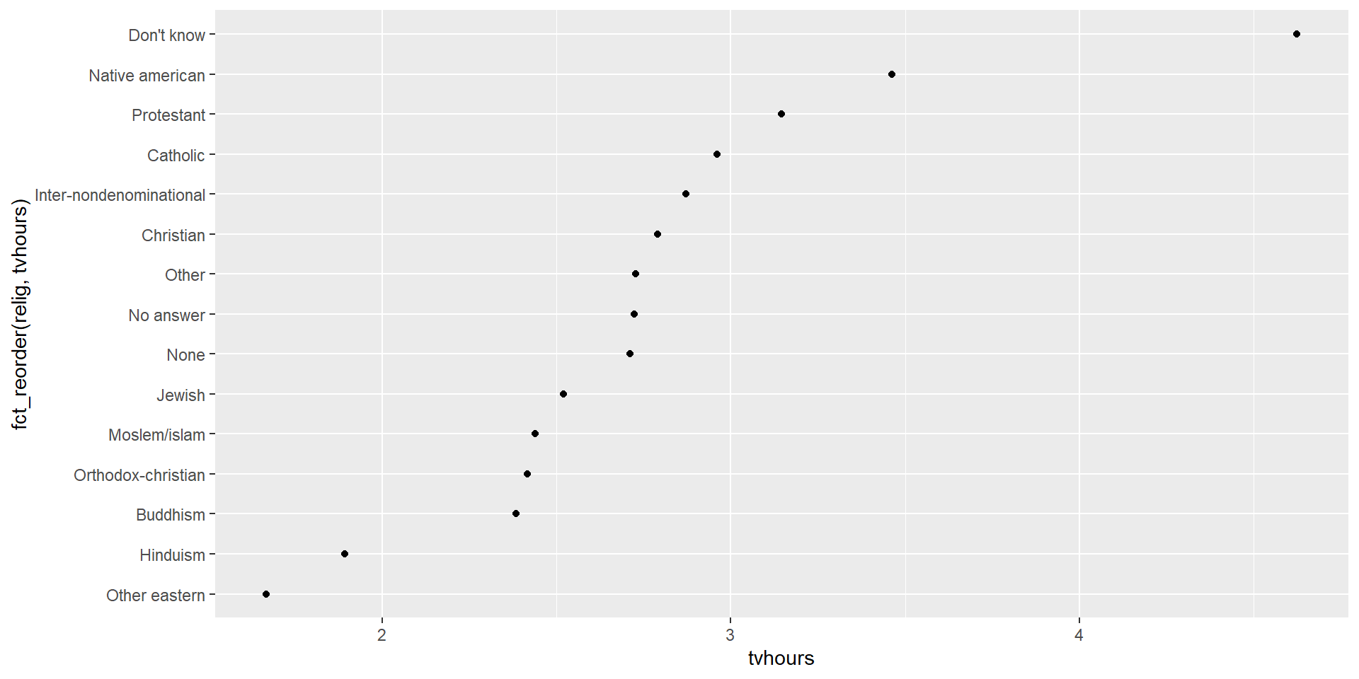
A scatterplot of with tvhours on the x-axis and religion on the y-axis. The y-axis is ordered seemingly aribtrarily making it hard to get any sense of overall pattern.

Factor reorder

It is hard to read this plot because there’s no overall pattern. We can improve it by reordering the levels of relig using fct_reorder(). fct_reorder() takes three arguments:

  • .f, the factor whose levels you want to modify.
  • .x, a numeric vector that you want to use to reorder the levels.
  • Optionally, .fun, a function that’s used if there are mu
ggplot(relig_summary, aes(x = tvhours, y = fct_reorder(relig, tvhours))) +
  geom_point()
The same scatterplot as above, but now the religion is displayed in increasing order of tvhours. "Other eastern" has the fewest tvhours under 2, and "Don't know" has the highest (over 5).

Factor reorder

The same scatterplot as above, but now the religion is displayed in increasing order of tvhours. "Other eastern" has the fewest tvhours under 2, and "Don't know" has the highest (over 5).

Factor relevel

Imagine the following plot, maybe you would like to have “Not applicable” not show up at the top of the graph.

A scatterplot with age on the x-axis and income on the y-axis. Income has been reordered in order of average age which doesn't make much sense. One section of the y-axis goes from $6000-6999, then <$1000, then $8000-9999.

Factor relevel

You can use fct_relevel(). It takes a factor, .f, and then any number of levels that you want to move to the front of the line.

ggplot(rincome_summary, aes(x = age, y = fct_relevel(rincome, "Not applicable"))) +
  geom_point()
The same scatterplot but now "Not Applicable" is displayed at the bottom of the y-axis. Generally there is a positive association between income and age, and the income band with the highethst average age is "Not applicable".

Other usefull refactoring functions

  • fct_reorder2(.f, .x, .y) reorders the factor .f by the .y values associated with the largest .x values.
  • fct_infreq() to order levels in decreasing frequency.
  • Combine it with fct_rev() if you want them in increasing frequency.
  • fct_recode() allows you to recode, or change, the value of each level.

Other usefull re-factoring functions

  • fct_collapse() is a useful variant of fct_recode() using a vector of old levels.
  • fct_lump_lowfreq() is a simple starting point that progressively lumps the smallest groups categories into “Other”, always keeping “Other” as the smallest category.
  • fct_lump_n() specifies the exact number of groups.