Decision Trees

Lecture 12

2025-04-17

Introduction to Decision Trees

Prerequisites

• This lecture will focus on Decision Trees and introduce Random Forests, powerful techniques for classification and regression tasks.
• We’ll use the rpart package for decision trees and the randomForest package for random forests.

# Install necessary packages if not already installed
if(!require(tidyverse)) install.packages("tidyverse")
if(!require(rpart)) install.packages("rpart")
if(!require(rpart.plot)) install.packages("rpart.plot") # Install rpart.plot
if(!require(caret)) install.packages("caret")
if(!require(randomForest)) install.packages("randomForest")
if(!require(DiagrammeR)) install.packages("DiagrammeR")

# Load the libraries
library(tidyverse)
library(rpart)
library(rpart.plot) # Load rpart.plot
library(caret)
library(randomForest)
library(DiagrammeR) # Load DiagrammeR

What are Decision Trees?

Decision Trees: An Intuitive Approach

Decision trees are a widely-used and intuitive machine learning technique used to solve prediction problems. They work through a series of yes-no questions to arrive at an outcome.

Some of the conceptual explanation here is inspired by Shaw Talebi’s excellent work on decision trees. For a Python-oriented approach, see his blog post.

A Simple Example

Imagine deciding whether to drink tea or coffee based on: - Time of day - Hours of sleep from last night

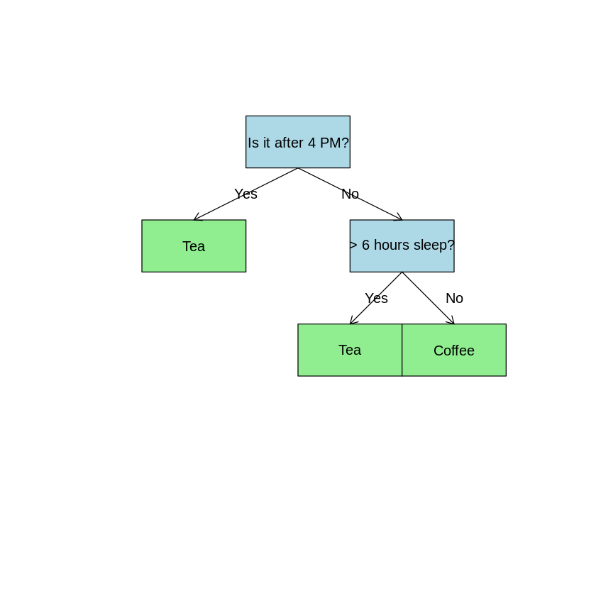
Simple decision tree example

Decision Tree Structure

A decision tree consists of:

• Root Node: The initial splitting point (Is it after 4 PM?)
• Internal/Splitting Nodes: Further split data based on conditions (Hours of sleep > 6?)
• Leaf/Terminal Nodes: Final outcome where no further splits occur (Tea 🍵 or Coffee ☕)
• Edges: Connect nodes and represent decision paths (Yes/No)

Using Decision Trees with Data

In practice, we use tabular data where each row is evaluated through the tree:

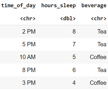
Tabular data example

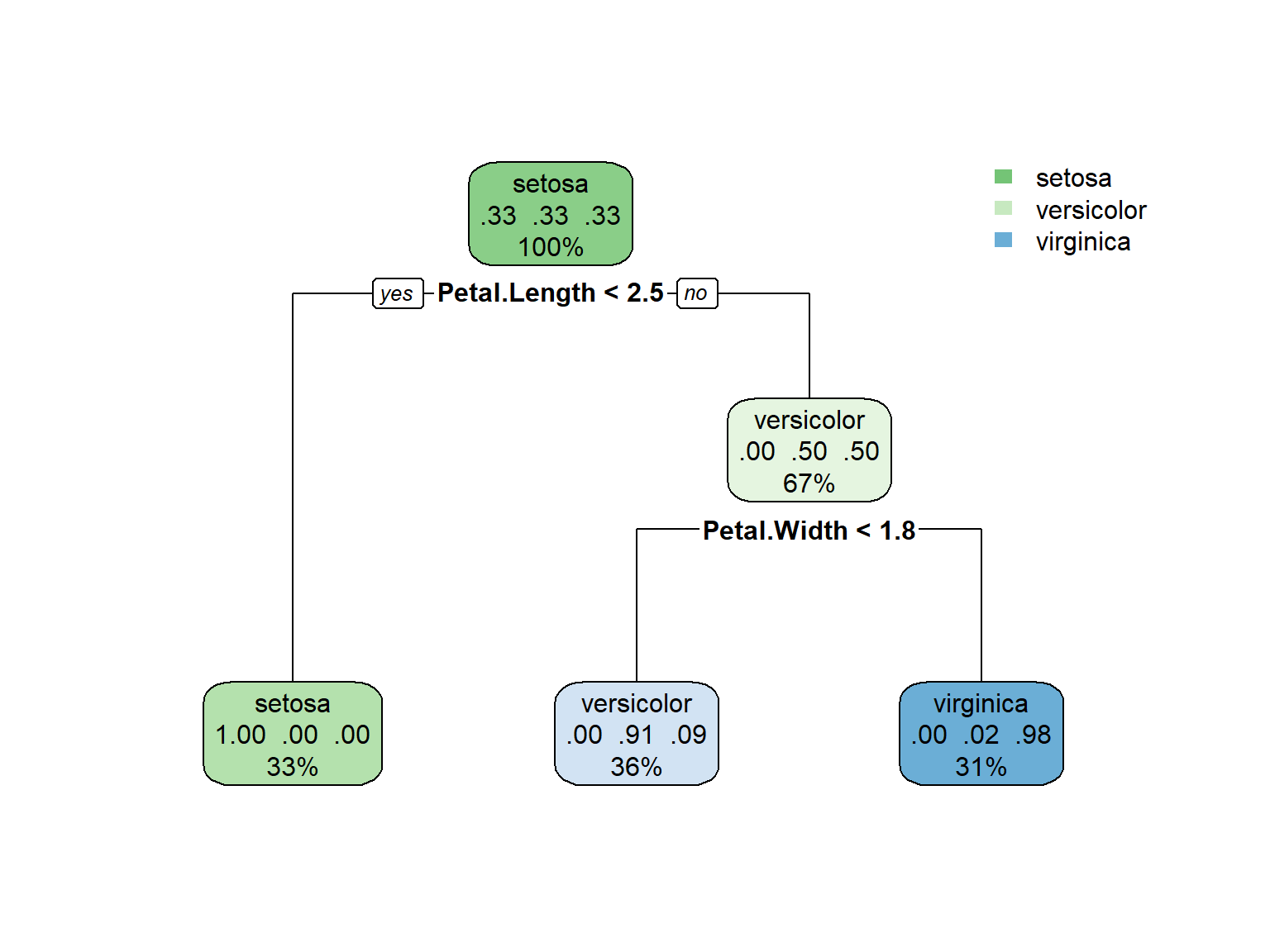
Graphical View of a Decision Tree

Decision trees partition the feature space into regions:

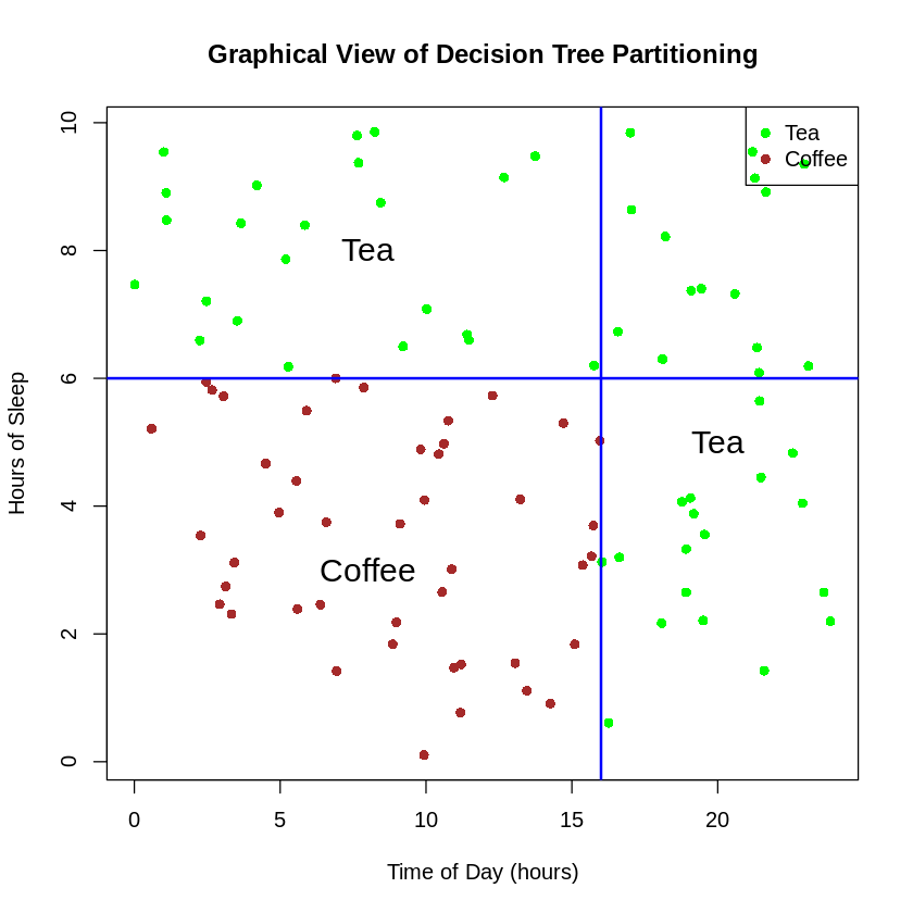
Graphical view of decision tree partitioning

How to Grow a Decision Tree

Training Decision Trees from Data

Decision trees are grown using an optimization process:

1. Starting Point: Begin with all data in a single node
2. Greedy Search: Find the “best” variable and splitting point
3. Recursive Splitting: Repeat the process on each resulting partition
4. Stopping: Continue until a stopping criterion is met

Split Criteria

Decision trees use various metrics to determine the best split:

• Classification Trees:
  • Gini impurity (default in many implementations)
  • Information gain / Entropy reduction
• Regression Trees:
  • Mean Squared Error (MSE)
  • Mean Absolute Error (MAE)

Overfitting in Decision Trees

A fully grown tree might perfectly classify training data but perform poorly on new data:

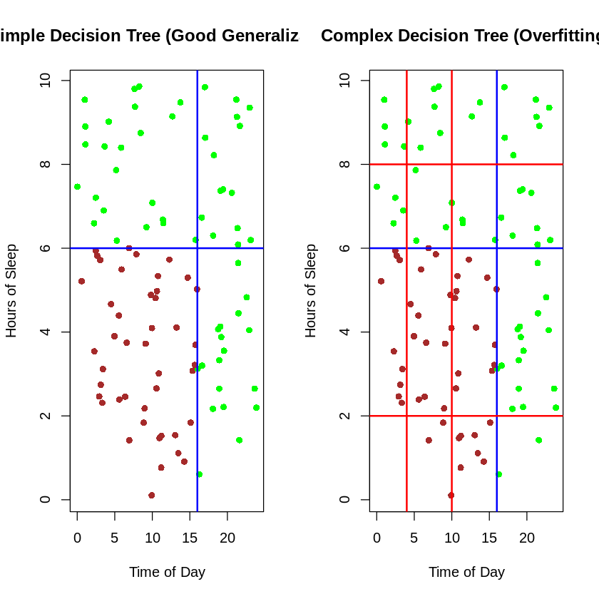
Comparison of simple vs. complex decision boundaries

Controlling Tree Growth

To prevent overfitting, we can use:

1. Hyperparameter Tuning:
   • Maximum tree depth
   • Minimum samples per leaf
   • Minimum samples for split
2. Pruning:
   • Grow a full tree, then remove branches that don’t improve performance
   • Cost-complexity pruning

Decision Trees in R

The rpart Package

R has excellent support for decision trees through the rpart package:

# Load a sample dataset - iris
data(iris)
head(iris)

  Sepal.Length Sepal.Width Petal.Length Petal.Width Species
1          5.1         3.5          1.4         0.2  setosa
2          4.9         3.0          1.4         0.2  setosa
3          4.7         3.2          1.3         0.2  setosa
4          4.6         3.1          1.5         0.2  setosa
5          5.0         3.6          1.4         0.2  setosa
6          5.4         3.9          1.7         0.4  setosa

Building a Simple Decision Tree

# Build a decision tree model
iris_tree <- rpart(Species ~ ., 
                  data = iris,
                  method = "class")

# Print the model
print(iris_tree)

n= 150 

node), split, n, loss, yval, (yprob)
      * denotes terminal node

1) root 150 100 setosa (0.33333333 0.33333333 0.33333333)  
  2) Petal.Length< 2.45 50   0 setosa (1.00000000 0.00000000 0.00000000) *
  3) Petal.Length>=2.45 100  50 versicolor (0.00000000 0.50000000 0.50000000)  
    6) Petal.Width< 1.75 54   5 versicolor (0.00000000 0.90740741 0.09259259) *
    7) Petal.Width>=1.75 46   1 virginica (0.00000000 0.02173913 0.97826087) *

Visualizing the Decision Tree

# Plot the decision tree
rpart.plot(iris_tree, 
           extra = 104,      # Show sample sizes and percentage
           box.palette = "GnBu", # Color scheme
           fallen.leaves = TRUE) # Align leaves

Interpreting the Tree

• At each node, we see:
  • The predicted class
  • The probability distribution
  • The percentage of observations
  • The splitting criterion
• For the iris dataset:
  • The first split is on Petal.Length < 2.5
  • This perfectly separates setosa from the other species
  • The second split uses Petal.Width to separate versicolor and virginica

Practical Example: Diabetes Prediction

Diabetes Dataset

Let’s use the Pima Indians Diabetes Dataset to predict diabetes risk:

# Load diabetes data
diabetes_data <- read.csv("https://raw.githubusercontent.com/jbrownlee/Datasets/master/pima-indians-diabetes.csv", header = FALSE)

# Set column names
colnames(diabetes_data) <- c("Pregnancies", "Glucose", "BloodPressure", "SkinThickness", 
                            "Insulin", "BMI", "DiabetesPedigreeFunction", "Age", "Outcome")

# Check the data
glimpse(diabetes_data)

Rows: 768
Columns: 9
$ Pregnancies              <int> 6, 1, 8, 1, 0, 5, 3, 10, 2, 8, 4, 10, 10, 1, …
$ Glucose                  <int> 148, 85, 183, 89, 137, 116, 78, 115, 197, 125…
$ BloodPressure            <int> 72, 66, 64, 66, 40, 74, 50, 0, 70, 96, 92, 74…
$ SkinThickness            <int> 35, 29, 0, 23, 35, 0, 32, 0, 45, 0, 0, 0, 0, …
$ Insulin                  <int> 0, 0, 0, 94, 168, 0, 88, 0, 543, 0, 0, 0, 0, …
$ BMI                      <dbl> 33.6, 26.6, 23.3, 28.1, 43.1, 25.6, 31.0, 35.…
$ DiabetesPedigreeFunction <dbl> 0.627, 0.351, 0.672, 0.167, 2.288, 0.201, 0.2…
$ Age                      <int> 50, 31, 32, 21, 33, 30, 26, 29, 53, 54, 30, 3…
$ Outcome                  <int> 1, 0, 1, 0, 1, 0, 1, 0, 1, 1, 0, 1, 0, 1, 1, …

Understanding the Dataset

The dataset contains information about females of Pima Indian heritage with the following variables:

• Pregnancies: Number of pregnancies
• Glucose: Plasma glucose concentration (2 hours after oral glucose tolerance test)
• BloodPressure: Diastolic blood pressure (mm Hg)
• SkinThickness: Triceps skin fold thickness (mm)
• Insulin: 2-Hour serum insulin (mu U/ml)
• BMI: Body mass index (weight in kg/(height in m)^2)
• DiabetesPedigreeFunction: A function of diabetes family history
• Age: Age in years
• Outcome: Class variable (0 = no diabetes, 1 = diabetes)

Preprocessing the Data

# Convert target to factor for classification
diabetes_data$Outcome <- as.factor(diabetes_data$Outcome)

# Recode target for interpretability
levels(diabetes_data$Outcome) <- c("Healthy", "Diabetic")

# Handle missing values (zeros are unlikely values for many of these measurements)
diabetes_data$Glucose[diabetes_data$Glucose == 0] <- NA
diabetes_data$BloodPressure[diabetes_data$BloodPressure == 0] <- NA
diabetes_data$SkinThickness[diabetes_data$SkinThickness == 0] <- NA
diabetes_data$Insulin[diabetes_data$Insulin == 0] <- NA
diabetes_data$BMI[diabetes_data$BMI == 0] <- NA

# Impute missing values with median
for(i in 1:5) {
  diabetes_data[is.na(diabetes_data[,i+1]), i+1] <- median(diabetes_data[,i+1], na.rm = TRUE)
}

# Check class balance
table(diabetes_data$Outcome)

 Healthy Diabetic 
     500      268 

Data Preparation

# Split into training and testing sets
set.seed(123)
train_index <- createDataPartition(diabetes_data$Outcome, p = 0.7, list = FALSE)
train_data <- diabetes_data[train_index, ]
test_data <- diabetes_data[-train_index, ]

# Check class balance
prop.table(table(train_data$Outcome))

  Healthy  Diabetic 
0.6505576 0.3494424 

Training the Model

# Train a decision tree model
diabetes_tree <- rpart(Outcome ~ ., 
                      data = train_data,
                      method = "class",
                      control = rpart.control(cp = 0.01)) # complexity parameter

# View the result
rpart.plot(diabetes_tree, 
           extra = 106,      
           box.palette = "RdBu",
           fallen.leaves = TRUE,
           main = "Diabetes Classification Decision Tree")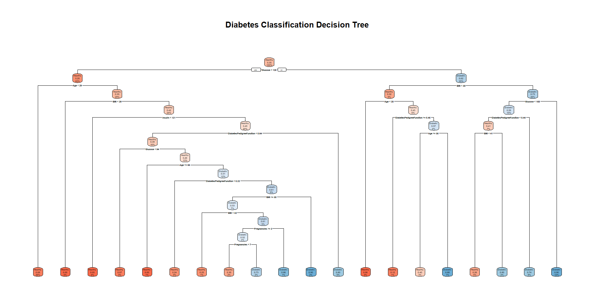

Evaluating the Model

# Make predictions on test data
predictions <- predict(diabetes_tree, test_data, type = "class")

# Create confusion matrix
conf_matrix <- confusionMatrix(predictions, test_data$Outcome)
conf_matrix

Confusion Matrix and Statistics

          Reference
Prediction Healthy Diabetic
  Healthy      134       35
  Diabetic      16       45
                                         
               Accuracy : 0.7783         
                 95% CI : (0.719, 0.8302)
    No Information Rate : 0.6522         
    P-Value [Acc > NIR] : 2.232e-05      
                                         
                  Kappa : 0.4826         
                                         
 Mcnemar's Test P-Value : 0.01172        
                                         
            Sensitivity : 0.8933         
            Specificity : 0.5625         
         Pos Pred Value : 0.7929         
         Neg Pred Value : 0.7377         
             Prevalence : 0.6522         
         Detection Rate : 0.5826         
   Detection Prevalence : 0.7348         
      Balanced Accuracy : 0.7279         
                                         
       'Positive' Class : Healthy        
                                         

Feature Importance

# Extract variable importance
var_importance <- diabetes_tree$variable.importance
var_importance_df <- data.frame(
  Variable = names(var_importance),
  Importance = var_importance
)

# Plot variable importance
ggplot(var_importance_df, aes(x = reorder(Variable, Importance), y = Importance)) +
  geom_bar(stat = "identity", fill = "steelblue") +
  coord_flip() +
  labs(x = "Variables", y = "Importance", 
       title = "Variable Importance in Diabetes Prediction") +
  theme_minimal()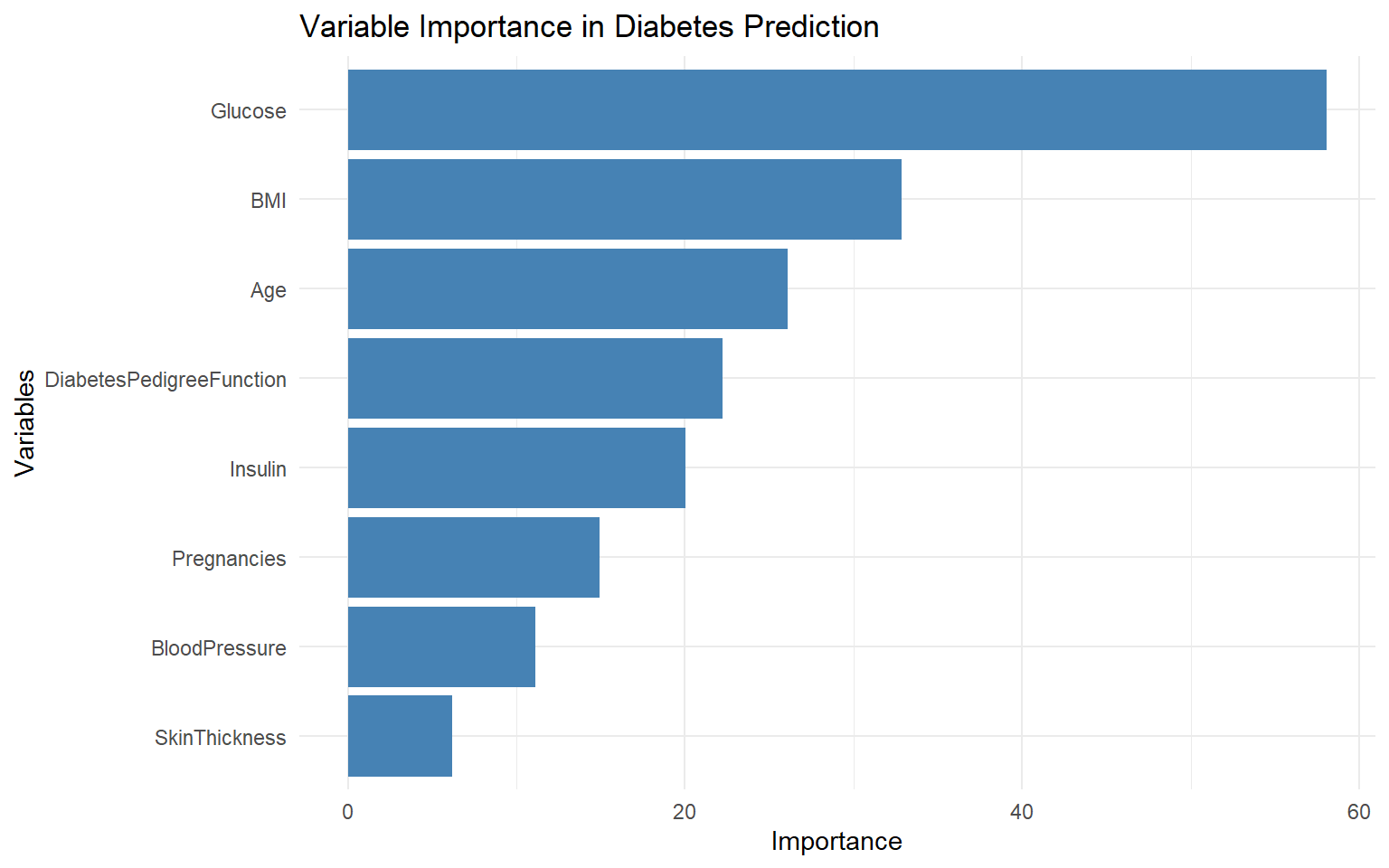

Hyperparameter Tuning

We can tune the complexity parameter (cp) to control tree growth:

# Plot cp values
plotcp(diabetes_tree)

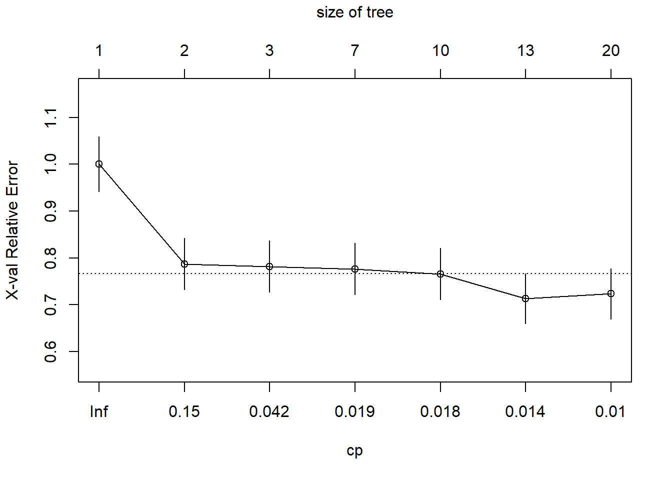
# Find optimal cp value
optimal_cp <- diabetes_tree$cptable[which.min(diabetes_tree$cptable[,"xerror"]),"CP"]
cat("Optimal CP value:", optimal_cp, "\n")

Optimal CP value: 0.0106383 

# Train model with optimal cp
pruned_tree <- prune(diabetes_tree, cp = optimal_cp)

# Plot pruned tree
rpart.plot(pruned_tree,
           extra = 106,
           box.palette = "RdBu",
           fallen.leaves = TRUE,
           main = "Pruned Diabetes Classification Tree")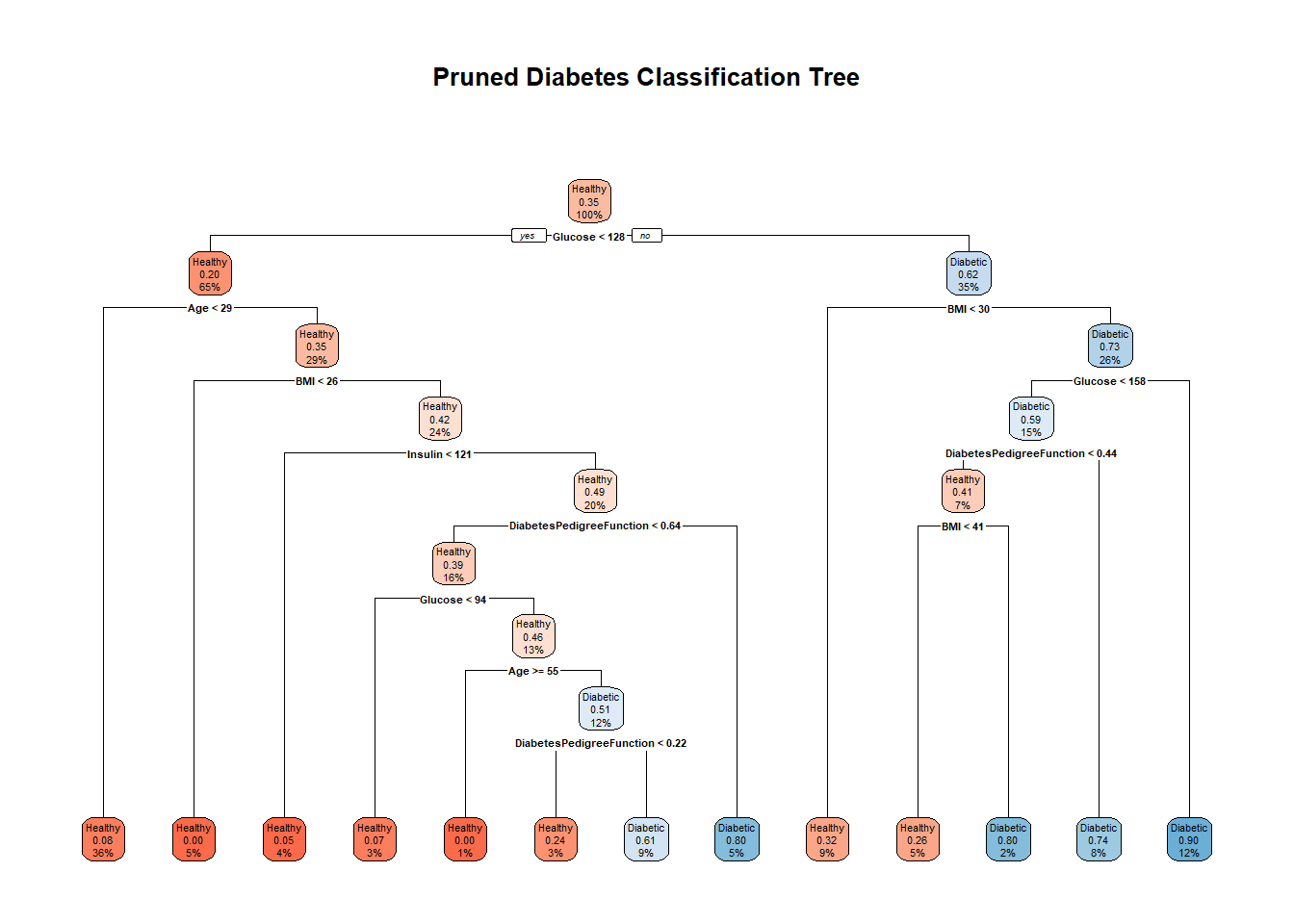

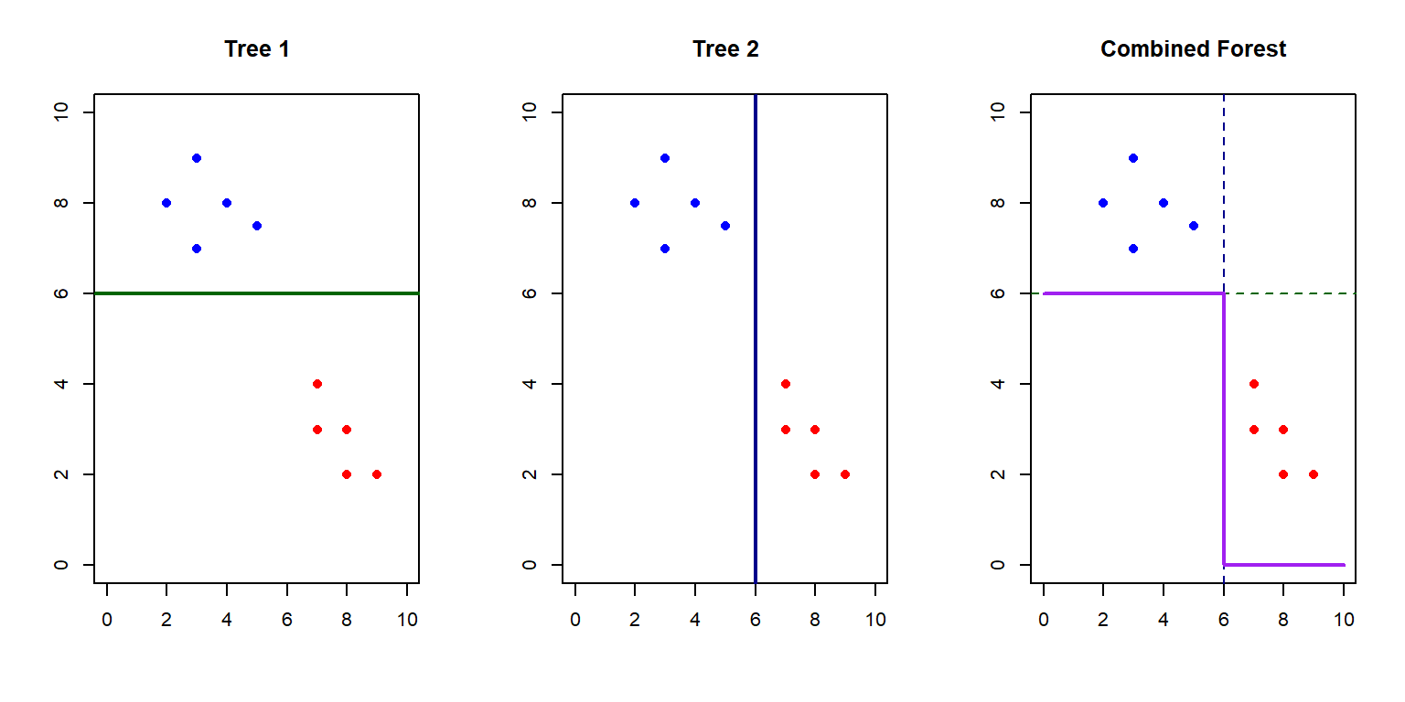
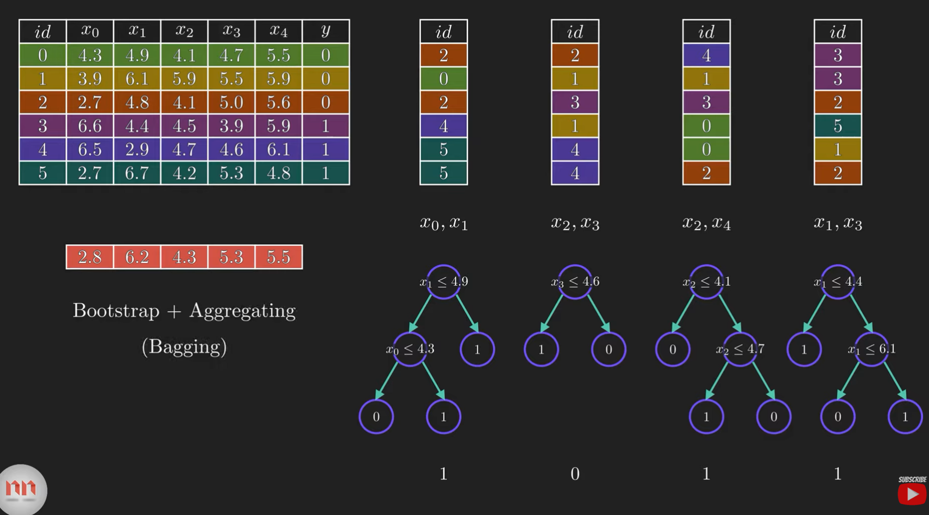
Model Comparison

# Evaluate pruned model
pruned_predictions <- predict(pruned_tree, test_data, type = "class")
pruned_conf_matrix <- confusionMatrix(pruned_predictions, test_data$Outcome)

# Compare metrics
metrics_comparison <- data.frame(
  Model = c("Full Tree", "Pruned Tree"),
  Accuracy = c(conf_matrix$overall["Accuracy"], 
               pruned_conf_matrix$overall["Accuracy"]),
  Sensitivity = c(conf_matrix$byClass["Sensitivity"], 
                  pruned_conf_matrix$byClass["Sensitivity"]),
  Specificity = c(conf_matrix$byClass["Specificity"], 
                  pruned_conf_matrix$byClass["Specificity"])
)

metrics_comparison

        Model  Accuracy Sensitivity Specificity
1   Full Tree 0.7782609   0.8933333      0.5625
2 Pruned Tree 0.7913043   0.8933333      0.6000

Advantages & Limitations

Advantages of Decision Trees

• Interpretability: Easy to understand and visualize
• No scaling required: Doesn’t require feature normalization
• Handles mixed data types: Can process numerical and categorical variables
• Captures non-linear relationships: Can model complex decision boundaries
• Feature importance: Naturally reveals important variables

Limitations of Decision Trees

• Overfitting: Prone to capturing noise in training data
• Instability: Small changes in data can result in very different trees
• Bias toward variables with many levels: Can favor categorical variables with many categories
• Suboptimal global decisions: Greedy approach may not find globally optimal tree
• Limited prediction smoothness: Step-wise predictions rather than smooth functions

Introduction to Random Forests

Ensemble Learning

Random Forests overcome many limitations of single decision trees through:

• Bootstrap Aggregation (Bagging): Training many trees on random subsets of data
• Feature Randomization: Considering only a subset of features at each split
• Voting/Averaging: Combining predictions from all trees

Random Forest Intuitive Implementation

Random Forest Implementation

# Train Random Forest model
set.seed(123)
diabetes_rf <- randomForest(Outcome ~ ., 
                           data = train_data,
                           ntree = 100,    # Number of trees
                           mtry = sqrt(ncol(train_data)-1)) # Number of variables tried at each split

# Print the model
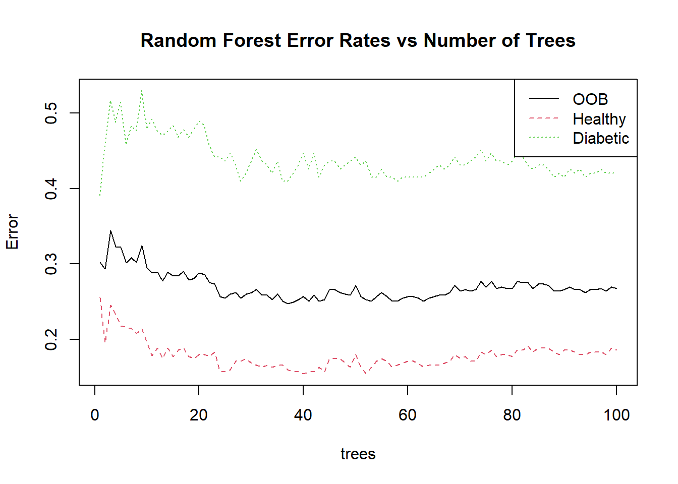
print(diabetes_rf)

Call:
 randomForest(formula = Outcome ~ ., data = train_data, ntree = 100,      mtry = sqrt(ncol(train_data) - 1)) 
               Type of random forest: classification
                     Number of trees: 100
No. of variables tried at each split: 3

        OOB estimate of  error rate: 26.77%
Confusion matrix:
         Healthy Diabetic class.error
Healthy      285       65   0.1857143
Diabetic      79      109   0.4202128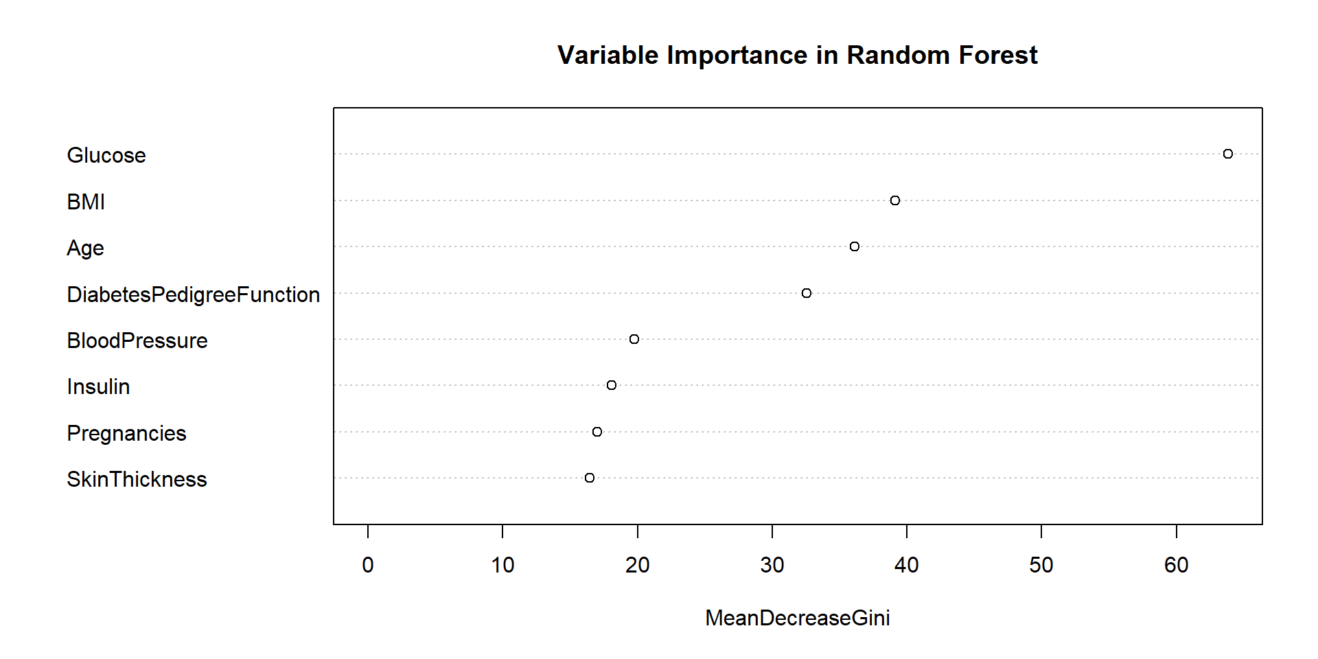

# Variable importance
varImpPlot(diabetes_rf, main = "Variable Importance in Random Forest")

Random Forest Performance

# Make predictions
rf_predictions <- predict(diabetes_rf, test_data)
rf_conf_matrix <- confusionMatrix(rf_predictions, test_data$Outcome)

# Add to comparison
metrics_comparison <- rbind(metrics_comparison,
                           data.frame(
                             Model = "Random Forest",
                             Accuracy = rf_conf_matrix$overall["Accuracy"],
                             Sensitivity = rf_conf_matrix$byClass["Sensitivity"],
                             Specificity = rf_conf_matrix$byClass["Specificity"]
                           ))

metrics_comparison

                 Model  Accuracy Sensitivity Specificity
1            Full Tree 0.7782609   0.8933333      0.5625
2          Pruned Tree 0.7913043   0.8933333      0.6000
Accuracy Random Forest 0.7608696   0.8533333      0.5875

Out-of-Bag Error Estimation

One unique advantage of Random Forests is out-of-bag (OOB) error estimation:

# Plot error vs number of trees
plot(diabetes_rf, main = "Random Forest Error Rates vs Number of Trees")
legend("topright", colnames(diabetes_rf$err.rate), col = 1:3, lty = 1:3)

Advanced Topics

Tree Ensembles Beyond Random Forests

Other tree-based ensemble methods include:

• Gradient Boosting: Builds trees sequentially, each correcting errors of previous trees
  • XGBoost, LightGBM, CatBoost
• AdaBoost: Boosts performance by giving higher weight to misclassified instances
• Extremely Randomized Trees: Adds additional randomization in splitting

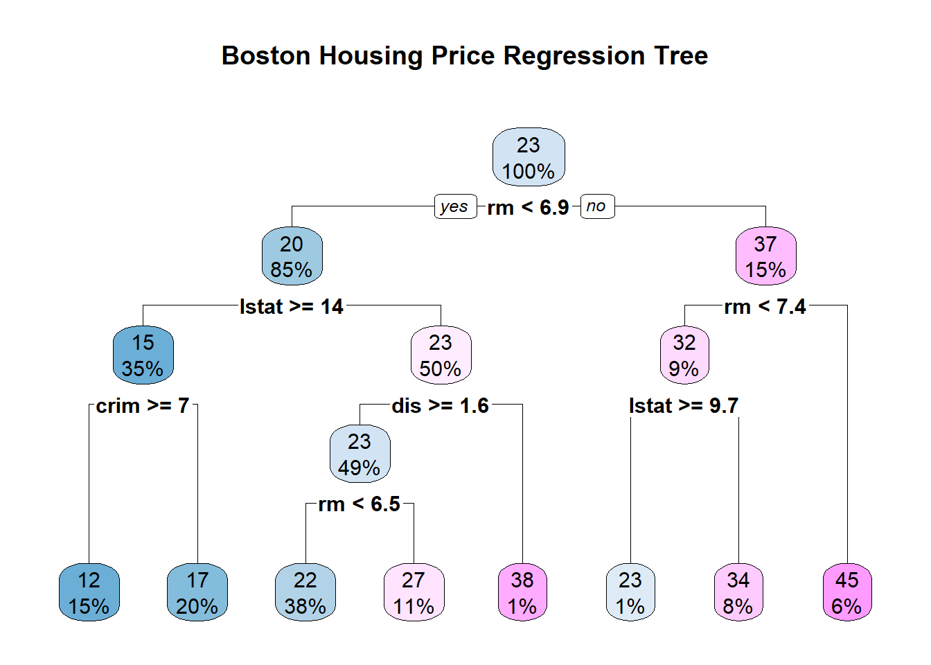
Regression Trees

Decision trees can also be used for regression problems:

# Create a simple regression tree example
data(Boston, package = "MASS")

# Train a regression tree
boston_tree <- rpart(medv ~ ., data = Boston)

# Plot the regression tree
rpart.plot(boston_tree, 
           main = "Boston Housing Price Regression Tree",
           box.palette = "BuPu")

Conclusion

Summary

• Decision trees provide an intuitive approach to classification and regression
• They work by recursively partitioning data based on feature values
• Controlling tree growth is crucial to prevent overfitting
• Random forests improve performance by combining many trees
• Both algorithms provide interpretable models with built-in feature importance

Key Takeaways

1. Decision trees are excellent for initial modeling and understanding data
2. Hyperparameter tuning and pruning help prevent overfitting
3. Random forests generally outperform single decision trees
4. Consider the tradeoff between interpretability and performance
5. These techniques work well across many domains and data types

References

1. Talebi, S. (2023). “Decision Trees: Introduction & Intuition”. Medium
2. Breiman, L., Friedman, J., Stone, C.J., & Olshen, R.A. (1984). “Classification and Regression Trees”
3. Breiman, L. (2001). “Random Forests”. Machine Learning, 45(1), 5-32
4. James, G., Witten, D., Hastie, T., & Tibshirani, R. (2013). “An Introduction to Statistical Learning”
5. Smith, J.W., Everhart, J.E., Dickson, W.C., Knowler, W.C., & Johannes, R.S. (1988). “Using the ADAP learning algorithm to forecast the onset of diabetes mellitus”
6. Normalized Nerd. (2022). “Random Forest Algorithm Clearly Explained!”. (https://www.youtube.com/watch?v=v6VJ2RO66Ag&ab_channel=NormalizedNerd)

Thank You!

Questions?

Feel free to reach out with any questions about decision trees or random forests!

R version 4.4.0 (2024-04-24 ucrt)
Platform: x86_64-w64-mingw32/x64
Running under: Windows 11 x64 (build 22631)

Matrix products: default


locale:
[1] LC_COLLATE=English_United States.utf8 
[2] LC_CTYPE=English_United States.utf8   
[3] LC_MONETARY=English_United States.utf8
[4] LC_NUMERIC=C                          
[5] LC_TIME=English_United States.utf8    

time zone: America/New_York
tzcode source: internal

attached base packages:
[1] stats     graphics  grDevices datasets  utils     methods   base     

other attached packages:
 [1] DiagrammeR_1.0.11    randomForest_4.7-1.2 caret_7.0-1         
 [4] lattice_0.22-6       rpart.plot_3.1.2     rpart_4.1.23        
 [7] lubridate_1.9.4      forcats_1.0.0        stringr_1.5.1       
[10] dplyr_1.1.4          purrr_1.0.4          readr_2.1.5         
[13] tidyr_1.3.1          tibble_3.2.1         ggplot2_3.5.1       
[16] tidyverse_2.0.0     

loaded via a namespace (and not attached):
 [1] tidyselect_1.2.1     timeDate_4041.110    farver_2.1.2        
 [4] fastmap_1.2.0        pROC_1.18.5          digest_0.6.36       
 [7] timechange_0.3.0     lifecycle_1.0.4      survival_3.5-8      
[10] magrittr_2.0.3       compiler_4.4.0       rlang_1.1.5         
[13] tools_4.4.0          yaml_2.3.10          data.table_1.17.0   
[16] knitr_1.48           labeling_0.4.3       htmlwidgets_1.6.4   
[19] plyr_1.8.9           RColorBrewer_1.1-3   withr_3.0.2         
[22] nnet_7.3-19          grid_4.4.0           stats4_4.4.0        
[25] e1071_1.7-16         colorspace_2.1-1     future_1.34.0       
[28] globals_0.16.3       scales_1.3.0         iterators_1.0.14    
[31] MASS_7.3-60.2        cli_3.6.4            rmarkdown_2.27      
[34] generics_0.1.3       rstudioapi_0.17.1    future.apply_1.11.3 
[37] reshape2_1.4.4       tzdb_0.5.0           visNetwork_2.1.2    
[40] proxy_0.4-27         splines_4.4.0        parallel_4.4.0      
[43] vctrs_0.6.5          hardhat_1.4.1        Matrix_1.7-0        
[46] jsonlite_1.8.8       hms_1.1.3            listenv_0.9.1       
[49] foreach_1.5.2        gower_1.0.2          recipes_1.2.0       
[52] glue_1.7.0           parallelly_1.43.0    codetools_0.2-20    
[55] stringi_1.8.4        gtable_0.3.6         munsell_0.5.1       
[58] pillar_1.10.1        htmltools_0.5.8.1    ipred_0.9-15        
[61] lava_1.8.1           R6_2.5.1             evaluate_0.24.0     
[64] renv_1.1.4           class_7.3-22         Rcpp_1.0.14         
[67] nlme_3.1-164         prodlim_2024.06.25   xfun_0.45           
[70] pkgconfig_2.0.3      ModelMetrics_1.2.2.2