Linear regression with a single predictor

Lecture 4

2025-02-10

Warm up

Goals

• Modeling with a single predictor
• Model parameters, estimates, and error terms
• Interpreting slopes and intercepts

Setup

Correlation vs. causation

Spurious correlations

Source: tylervigen.com/spurious-correlations

Spurious correlations

Source: tylervigen.com/spurious-correlations

Linear regression with a single predictor

Read the data

df_raw_cattle_numbers <- read.csv('https://raw.githubusercontent.com/Bovi-analytics/minor-digital-agriculture/refs/heads/main/data/fao-cattle-numbers.csv')

Data prep

• Select columns needed : Year and Value
• Apply correct FAIR naming convention

df_cattle_numbers <- df_raw_cattle_numbers %>%
  dplyr::select(Year, Value) %>%
  dplyr::rename(
    NumberOfCows = Value
  )

Data grouping

• Create a groupby Year
• Create sum for entire world

df_total_cattle_numbers <- df_cattle_numbers %>%
  dplyr::group_by(Year) %>%
  dplyr::summarise(
    TotalNumberOfCows = sum(NumberOfCows)/1000000000
  )

Writing the data

• Write the data to csv
• Import in Tableau

write_csv(df_total_cattle_numbers, file = "df_total_cattle_numbers.csv")

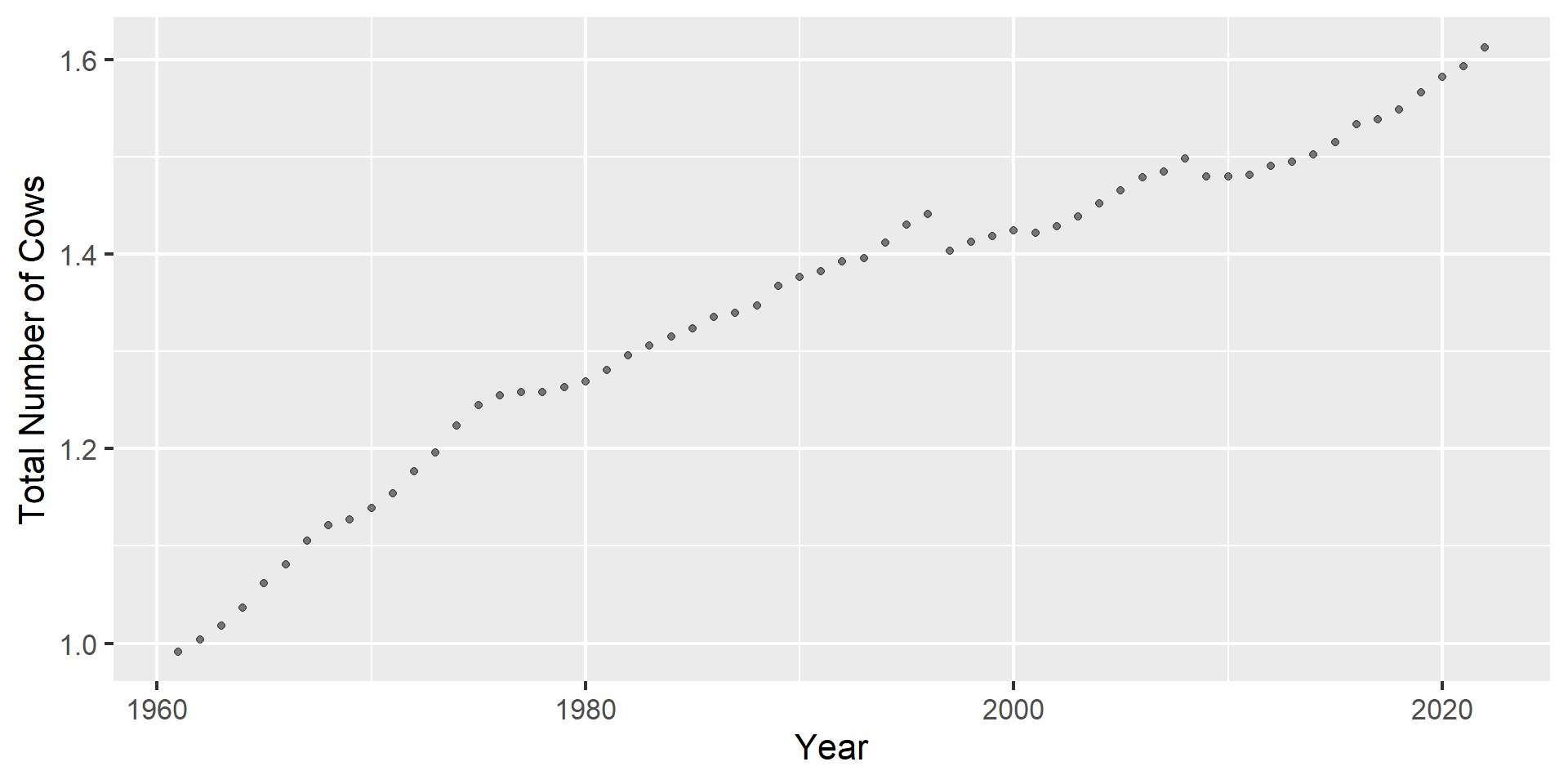
Data overview

df_total_cattle_numbers %>%
  select(Year, TotalNumberOfCows)

# A tibble: 62 × 2
    Year TotalNumberOfCows
   <int>             <dbl>
 1  1961             0.992
 2  1962             1.00 
 3  1963             1.02 
 4  1964             1.04 
 5  1965             1.06 
 6  1966             1.08 
 7  1967             1.11 
 8  1968             1.12 
 9  1969             1.13 
10  1970             1.14 
# ℹ 52 more rows

Data visualization

Regression model

A regression model is a function that describes the relationship between the outcome, \(Y\), and the predictor, \(X\).

\[\begin{aligned} Y &= \color{black}{\textbf{Model}} + \text{Error} \\[8pt] &= \color{black}{\mathbf{f(X)}} + \epsilon \\[8pt] &= \color{black}{\boldsymbol{\mu_{Y|X}}} + \epsilon \end{aligned}\]

Regression model

\[ \begin{aligned} Y &= \color{#325b74}{\textbf{Model}} + \text{Error} \\[8pt] &= \color{#325b74}{\mathbf{f(X)}} + \epsilon \\[8pt] &= \color{#325b74}{\boldsymbol{\mu_{Y|X}}} + \epsilon \end{aligned} \]

Simple linear regression

Use simple linear regression to model the relationship between a quantitative outcome (\(Y\)) and a single quantitative predictor (\(X\)): \[\Large{Y = \beta_0 + \beta_1 X + \epsilon}\]

• \(\beta_1\): True slope of the relationship between \(X\) and \(Y\)
• \(\beta_0\): True intercept of the relationship between \(X\) and \(Y\)
• \(\epsilon\): Error (residual)

Simple linear regression

\[\Large{\hat{Y} = b_0 + b_1 X}\]

• \(b_1\): Estimated slope of the relationship between \(X\) and \(Y\)
• \(b_0\): Estimated intercept of the relationship between \(X\) and \(Y\)
• No error term!

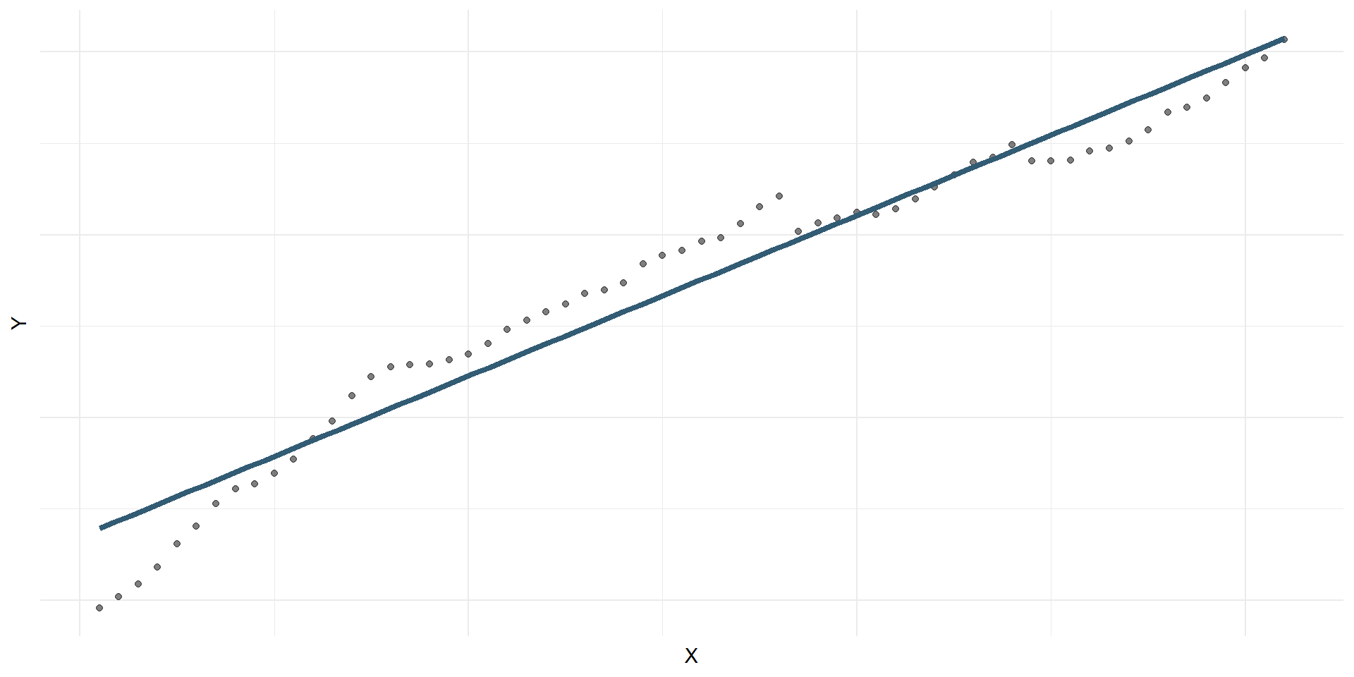
Choosing values for \(b_1\) and \(b_0\)

Residuals

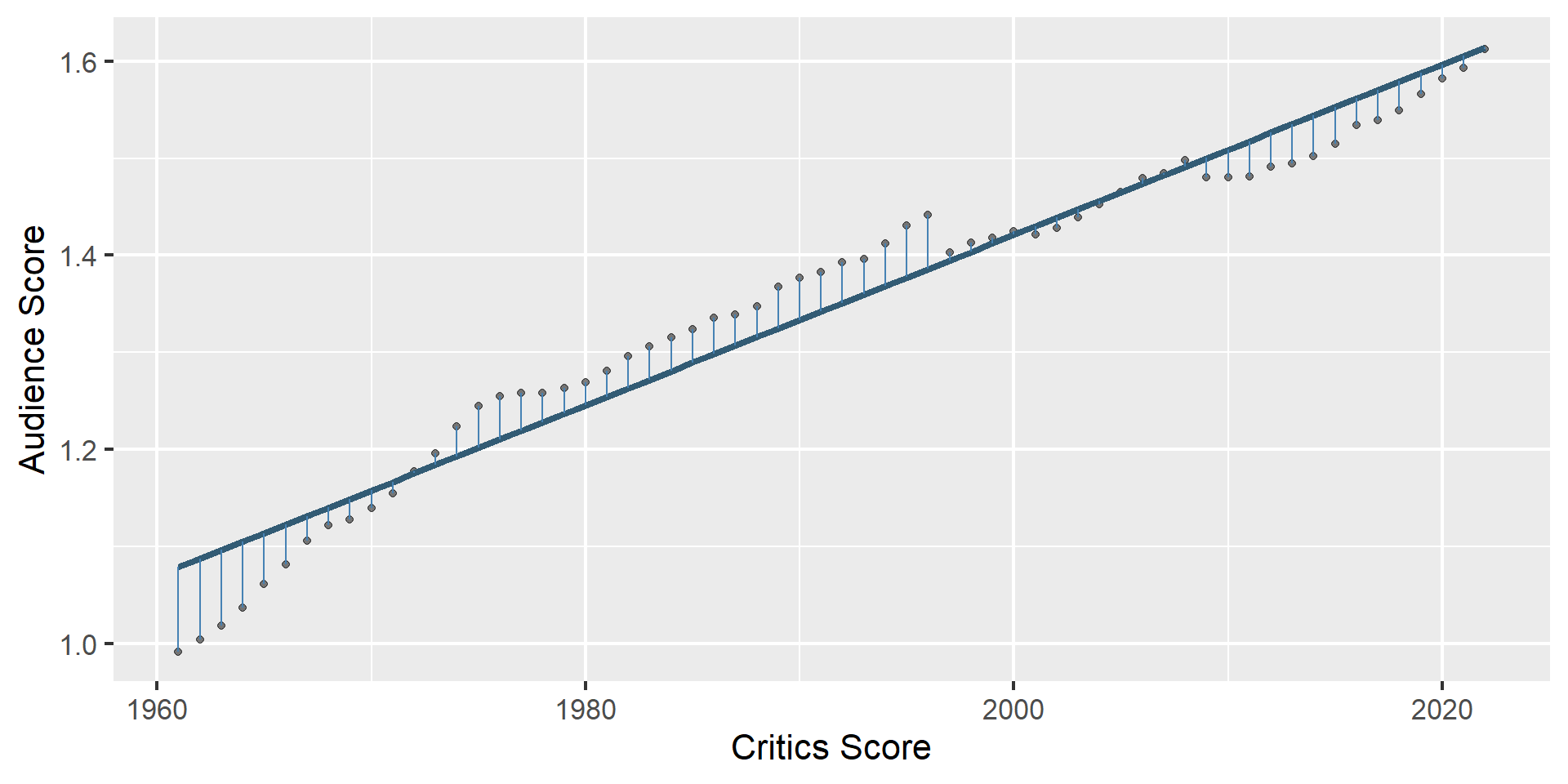
\[\text{residual} = \text{observed} - \text{predicted} = y - \hat{y}\]

Least squares line

• The residual for the \(i^{th}\) observation is

\[e_i = \text{observed} - \text{predicted} = y_i - \hat{y}_i\]

• The sum of squared residuals is

\[e^2_1 + e^2_2 + \dots + e^2_n\]

• The least squares line is the one that minimizes the sum of squared residuals

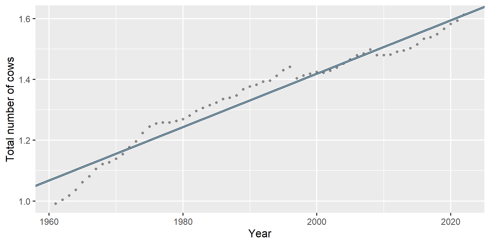
Least squares line

# A tibble: 2 × 5
  term         estimate std.error statistic  p.value
  <chr>           <dbl>     <dbl>     <dbl>    <dbl>
1 (Intercept) -16.1      0.510        -31.7 3.85e-39
2 Year          0.00879  0.000256      34.3 4.03e-41

Slope and intercept

Properties of least squares regression

• The regression line goes through the center of mass point (the coordinates corresponding to average \(X\) and average \(Y\)): \(b_0 = \bar{Y} - b_1~\bar{X}\)

• Slope has the same sign as the correlation coefficient: \(b_1 = r \frac{s_Y}{s_X}\)

• Sum of the residuals is zero: \(\sum_{i = 1}^n \epsilon_i = 0\)

• Residuals and \(X\) values are uncorrelated

Interpreting the slope

• Question
• Submit

The slope of the model for predicting number of cows is 0.008785434.

How to interpret

Interpreting slope & intercept

\[\widehat{\text{Total number of cows}} = -16.1 + 0.008785434 \times \text{Year}\]

• Slope: For every one point increase in Year, we expect the total number of cows to be higher by 0.008785434 points, on average.
• Intercept: In Year is 0, we expect the total number of cows to be -16.1.

Is the intercept meaningful?

✅ The intercept is meaningful in context of the data if

• the predictor can feasibly take values equal to or near zero or
• the predictor has values near zero in the observed data

🛑 Otherwise, it might not be meaningful!