Linear regression with multiple predictors

Lecture 5 - part A

2025-02-24

#Introduction

Goals

Recap on modeling with one predictor
Modeling with two predictors
Interpreting slopes and intercepts
Interpreting interactions

Setup

library(dplyr)
library(tidyverse)
library(tidymodels)
library(jtools)
library(sjPlot)
library(sjmisc)
ggplot2::theme_set(theme_gray(base_size = 16))

Linear regression with a single predictor

Simple linear regression

Use simple linear regression to model the relationship between a quantitative outcome (\(Y\)) and a single quantitative predictor (\(X\)): \[\Large{Y = \beta_0 + \beta_1 X + \epsilon}\]

\(\beta_1\): True slope of the relationship between \(X\) and \(Y\)
\(\beta_0\): True intercept of the relationship between \(X\) and \(Y\)
\(\epsilon\): Error (residual)

Interpreting slope & intercept

\[\widehat{\text{Total number of cows}} = -16.1 + 0.008785434 \times \text{Year}\]

Slope: For every one point increase in Year, we expect the total number of cows to be higher by 0.008785434 points, on average.
Intercept: In Year is 0, we expect the total number of cows to be -16.1.

Linear regression with a multiple predictors

Read the data

df_raw_cattle_numbers <- read.csv('https://raw.githubusercontent.com/Bovi-analytics/minor-digital-agriculture/refs/heads/main/data/fao-cattle-numbers.csv')

Data prep

Select columns Year, Area and Value
Apply correct FAIR naming convention
Mutate NumberOfCows to be easier to interpret
Filter specific countries

df_cattle_numbers <- df_raw_cattle_numbers %>%
  dplyr::rename(
    Country = Area,
    NumberOfCows = Value
  )  %>%
  dplyr::mutate(
    NumberOfCows =  NumberOfCows/1000000
  ) %>%
  dplyr::select(Year, Country, NumberOfCows) %>%
  dplyr::filter(
    Country %in% c("Brazil", "United States of America", "India")
  )

Data overview

df_cattle_numbers %>%
  select(Year, Country, NumberOfCows)

    Year                  Country NumberOfCows
1   1961                   Brazil     56.04131
2   1962                   Brazil     57.73989
3   1963                   Brazil     59.70304
4   1964                   Brazil     61.73294
5   1965                   Brazil     63.83186
6   1966                   Brazil     66.00214
7   1967                   Brazil     68.24622
8   1968                   Brazil     70.56661
9   1969                   Brazil     72.96586
10  1970                   Brazil     75.44670
11  1971                   Brazil     78.56226
12  1972                   Brazil     83.00000
13  1973                   Brazil     85.50000
14  1974                   Brazil     90.43701
15  1975                   Brazil     92.49536
16  1976                   Brazil    101.67400
17  1977                   Brazil    107.29656
18  1978                   Brazil    106.94256
19  1979                   Brazil    109.17749
20  1980                   Brazil    118.97142
21  1981                   Brazil    121.78501
22  1982                   Brazil    123.48800
23  1983                   Brazil    124.18600
24  1984                   Brazil    127.65501
25  1985                   Brazil    128.42267
26  1986                   Brazil    132.22157
27  1987                   Brazil    135.72029
28  1988                   Brazil    139.59910
29  1989                   Brazil    144.15410
30  1990                   Brazil    147.10232
31  1991                   Brazil    152.13550
32  1992                   Brazil    154.22930
33  1993                   Brazil    155.13407
34  1994                   Brazil    158.24323
35  1995                   Brazil    161.22794
36  1996                   Brazil    158.28854
37  1997                   Brazil    161.41616
38  1998                   Brazil    163.15436
39  1999                   Brazil    164.62104
40  2000                   Brazil    169.87552
41  2001                   Brazil    176.38873
42  2002                   Brazil    185.34884
43  2003                   Brazil    195.55158
44  2004                   Brazil    204.51274
45  2005                   Brazil    207.15670
46  2006                   Brazil    205.88624
47  2007                   Brazil    199.75201
48  2008                   Brazil    202.30673
49  2009                   Brazil    205.30795
50  2010                   Brazil    209.54111
51  2011                   Brazil    212.81531
52  2012                   Brazil    211.27908
53  2013                   Brazil    211.76429
54  2014                   Brazil    212.36613
55  2015                   Brazil    215.22051
56  2016                   Brazil    218.19077
57  2017                   Brazil    215.00358
58  2018                   Brazil    213.80945
59  2019                   Brazil    215.00896
60  2020                   Brazil    217.83628
61  2021                   Brazil    224.60199
62  2022                   Brazil    234.35265
63  1961                    India    175.60000
64  1962                    India    173.90000
65  1963                    India    173.97101
66  1964                    India    175.80000
67  1965                    India    175.90000
68  1966                    India    176.21200
69  1967                    India    176.38400
70  1968                    India    176.73101
71  1969                    India    177.08600
72  1970                    India    177.44200
73  1971                    India    177.81400
74  1972                    India    178.38400
75  1973                    India    178.33101
76  1974                    India    178.58000
77  1975                    India    179.45701
78  1976                    India    180.35000
79  1977                    India    180.28600
80  1978                    India    181.99200
81  1979                    India    184.30000
82  1980                    India    186.50000
83  1981                    India    188.70000
84  1982                    India    192.45301
85  1983                    India    193.79701
86  1984                    India    195.15400
87  1985                    India    196.52000
88  1986                    India    197.89501
89  1987                    India    199.69501
90  1988                    India    200.65000
91  1989                    India    201.60000
92  1990                    India    202.50000
93  1991                    India    203.50000
94  1992                    India    204.58400
95  1993                    India    203.63400
96  1994                    India    202.68400
97  1995                    India    201.73400
98  1996                    India    200.78400
99  1997                    India    198.88200
100 1998                    India    196.53501
101 1999                    India    194.21600
102 2000                    India    191.92400
103 2001                    India    189.66000
104 2002                    India    187.42200
105 2003                    India    185.18099
106 2004                    India    188.57000
107 2005                    India    192.02099
108 2006                    India    195.53501
109 2007                    India    199.07501
110 2008                    India    197.44499
111 2009                    India    195.81501
112 2010                    India    194.18499
113 2011                    India    192.55501
114 2012                    India    190.90410
115 2013                    India    189.00000
116 2014                    India    187.00000
117 2015                    India    188.07519
118 2016                    India    189.15420
119 2017                    India    190.48526
120 2018                    India    191.95754
121 2019                    India    193.46287
122 2020                    India    194.90437
123 2021                    India    192.87987
124 2022                    India    193.60691
125 1961 United States of America     97.70000
126 1962 United States of America    100.36901
127 1963 United States of America    104.48800
128 1964 United States of America    107.90301
129 1965 United States of America    109.00000
130 1966 United States of America    108.86200
131 1967 United States of America    108.78301
132 1968 United States of America    109.37101
133 1969 United States of America    110.01501
134 1970 United States of America    112.36901
135 1971 United States of America    114.57800
136 1972 United States of America    117.86200
137 1973 United States of America    121.53901
138 1974 United States of America    127.78800
139 1975 United States of America    132.02800
140 1976 United States of America    127.98000
141 1977 United States of America    122.81000
142 1978 United States of America    116.37501
143 1979 United States of America    110.86400
144 1980 United States of America    111.24200
145 1981 United States of America    114.35101
146 1982 United States of America    115.44400
147 1983 United States of America    115.00101
148 1984 United States of America    113.36000
149 1985 United States of America    109.58200
150 1986 United States of America    105.37800
151 1987 United States of America    102.11800
152 1988 United States of America     99.62200
153 1989 United States of America     96.74000
154 1990 United States of America     95.81600
155 1991 United States of America     96.39300
156 1992 United States of America     97.55600
157 1993 United States of America     99.17590
158 1994 United States of America    100.97360
159 1995 United States of America    102.78520
160 1996 United States of America    103.54820
161 1997 United States of America    101.65570
162 1998 United States of America     99.74400
163 1999 United States of America     99.11500
164 2000 United States of America     98.19900
165 2001 United States of America     97.29750
166 2002 United States of America     96.72300
167 2003 United States of America     96.10000
168 2004 United States of America     94.88800
169 2005 United States of America     95.01800
170 2006 United States of America     96.70150
171 2007 United States of America     96.57300
172 2008 United States of America     96.03450
173 2009 United States of America     94.72100
174 2010 United States of America     94.08120
175 2011 United States of America     92.88740
176 2012 United States of America     91.16020
177 2013 United States of America     90.09520
178 2014 United States of America     88.52600
179 2015 United States of America     89.14300
180 2016 United States of America     91.88800
181 2017 United States of America     93.62460
182 2018 United States of America     94.29800
183 2019 United States of America     94.80470
184 2020 United States of America     93.79330
185 2021 United States of America     93.78950
186 2022 United States of America     92.07660

Data visualization

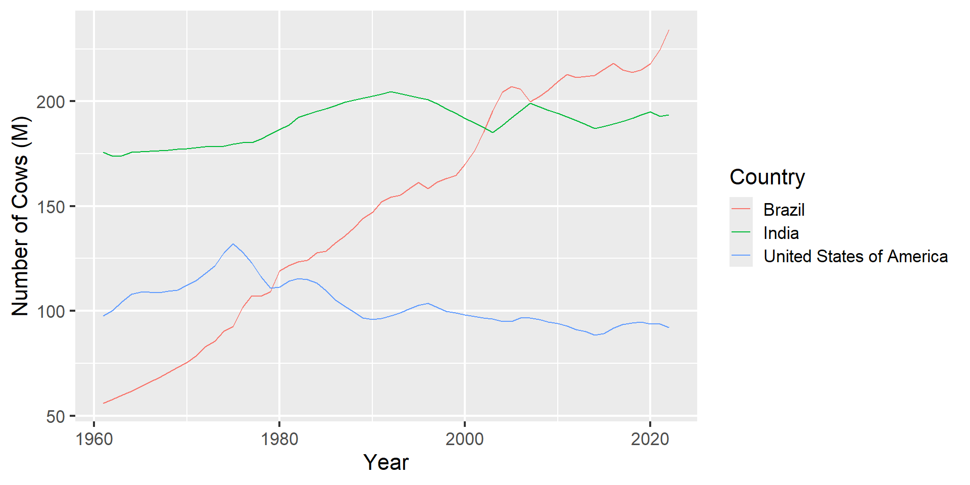
Regression model

m <- lm(NumberOfCows ~ Year + Country, data = df_cattle_numbers)

Multiple linear regression

Use multiple linear regression to model the relationship between a quantitative outcome (\(Y\)) and a multiple quantitative predictors and factors (\(X\)): \[\Large{Y = \beta_0 + \beta_1 X_1 + \beta_2 X_2 + \epsilon}\]

\(\beta_1\): True slope of the relationship between \(X_1\) and \(Y\)
\(\beta_2\): True slope of the relationship between \(X_2\) and \(Y\)
\(\beta_0\): True intercept of the relationship between \(X\) and \(Y\)
\(\epsilon\): Error (residual)

Multiple linear regression

cows_fit <- linear_reg() |>
  fit(NumberOfCows ~ Year + Country, data = df_cattle_numbers)

tidy(cows_fit)

# A tibble: 4 × 5
  term                             estimate std.error statistic  p.value
  <chr>                               <dbl>     <dbl>     <dbl>    <dbl>
1 (Intercept)                     -1785.      227.        -7.86 3.30e-13
2 Year                                0.970     0.114      8.51 6.39e-15
3 CountryIndia                       42.1       5.00       8.41 1.14e-14
4 CountryUnited States of America   -44.2       5.00      -8.84 8.12e-16

Is the intercept meaningful?

✅ The intercept is meaningful in context of the data if

the predictor can feasibly take values equal to or near zero or
the predictor has values near zero in the observed data

🛑 Otherwise, in this case not meaningful & difficult to interpret!

Make intercept more interpretable

Substract the initial value of year 1960 from each year value
How do you interpret the intercept of 116 now?
Did the slope for Year or Country change

cows_fit <- linear_reg() |>
  fit(
    NumberOfCows ~ Year + Country, 
    data = df_cattle_numbers %>% dplyr::mutate(Year = Year - 1960))
tidy(cows_fit)

# A tibble: 4 × 5
  term                            estimate std.error statistic  p.value
  <chr>                              <dbl>     <dbl>     <dbl>    <dbl>
1 (Intercept)                      117.        5.04      23.2  3.12e-56
2 Year                               0.970     0.114      8.51 6.39e-15
3 CountryIndia                      42.1       5.00       8.41 1.14e-14
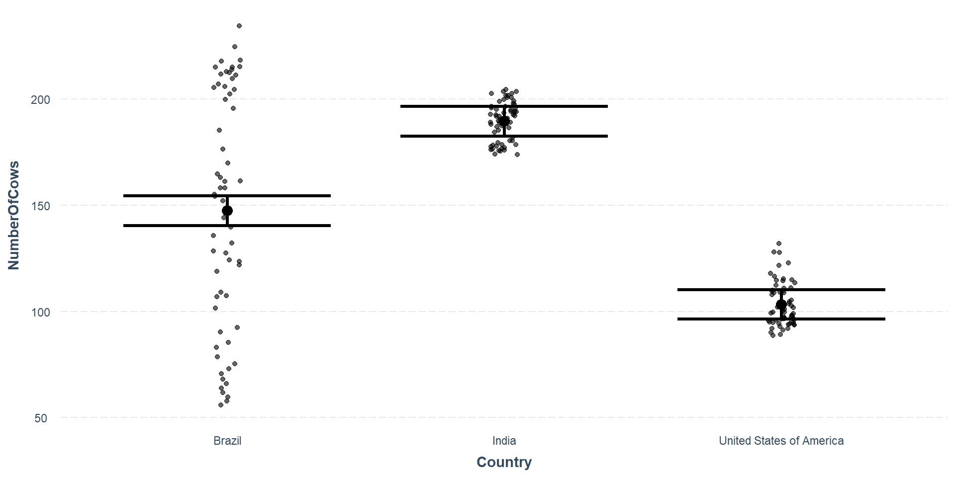
4 CountryUnited States of America  -44.2       5.00      -8.84 8.12e-16

Plot the slope effect of County

The estimate for India and USA was +42M and -44M

Plot the slope effect of Year

How do you interpret the slope of 0.97, combined with this graph?

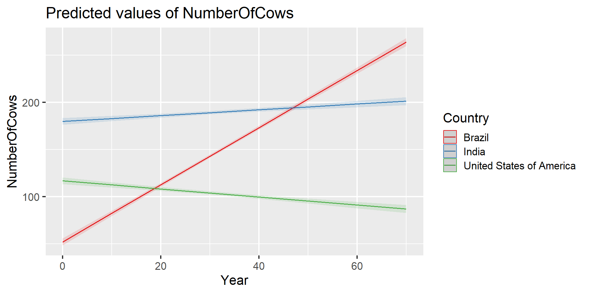
Linear regression with interaction

Code to introduce an interaction between predictors

Use * to make an interaction term

Year * Country or
Year + Country + Year:Country

MODEL INFO:
Observations: 186
Dependent Variable: NumberOfCows
Type: OLS linear regression 

MODEL FIT:
F(5,180) = 1642.26, p = 0.00
R² = 0.98
Adj. R² = 0.98 

Standard errors:OLS
----------------------------------------------------------------
                                     Est.   S.E.   t val.      p
-------------------------------- -------- ------ -------- ------
(Intercept)                         51.98   1.84    28.31   0.00
Year                                 3.03   0.05    59.82   0.00
CountryIndia                       127.86   2.60    49.25   0.00
CountryUnited States of             64.76   2.60    24.94   0.00
America                                                         
Year:CountryIndia                   -2.72   0.07   -38.00   0.00
Year:CountryUnited States of        -3.46   0.07   -48.26   0.00
America                                                         
----------------------------------------------------------------

Linear regression with multiple predictors

Goals

Setup

Linear regression with a single predictor

Simple linear regression

Interpreting slope & intercept

Linear regression with a multiple predictors

Read the data

Data prep

Data overview

Data visualization

Regression model

Multiple linear regression

Multiple linear regression

Is the intercept meaningful?

Make intercept more interpretable

Plot the slope effect of County

Plot the slope effect of Year

Linear regression with interaction

Code to introduce an interaction between predictors

Lets plot the interaction