── Attaching core tidyverse packages ──────────────────────── tidyverse 2.0.0 ──
✔ dplyr     1.1.4     ✔ readr     2.1.5
✔ forcats   1.0.0     ✔ stringr   1.5.1
✔ ggplot2   3.5.1     ✔ tibble    3.2.1
✔ lubridate 1.9.3     ✔ tidyr     1.3.1
✔ purrr     1.0.2
── Conflicts ────────────────────────────────────────── tidyverse_conflicts() ──
✖ dplyr::filter() masks stats::filter()
✖ dplyr::lag()    masks stats::lag()
ℹ Use the conflicted package (<http://conflicted.r-lib.org/>) to force all conflicts to become errorsData transformations
Lecture 8
2025-03-17
Warm up
Goals
It’s rare that all data is available in a dataframe to work with it. Typically you will have to manipulate data to get the data you want to analyse.
- Learn about the most important types of variables that you’ll encounter inside a data frame
- Learn the tools you can use to work with them.
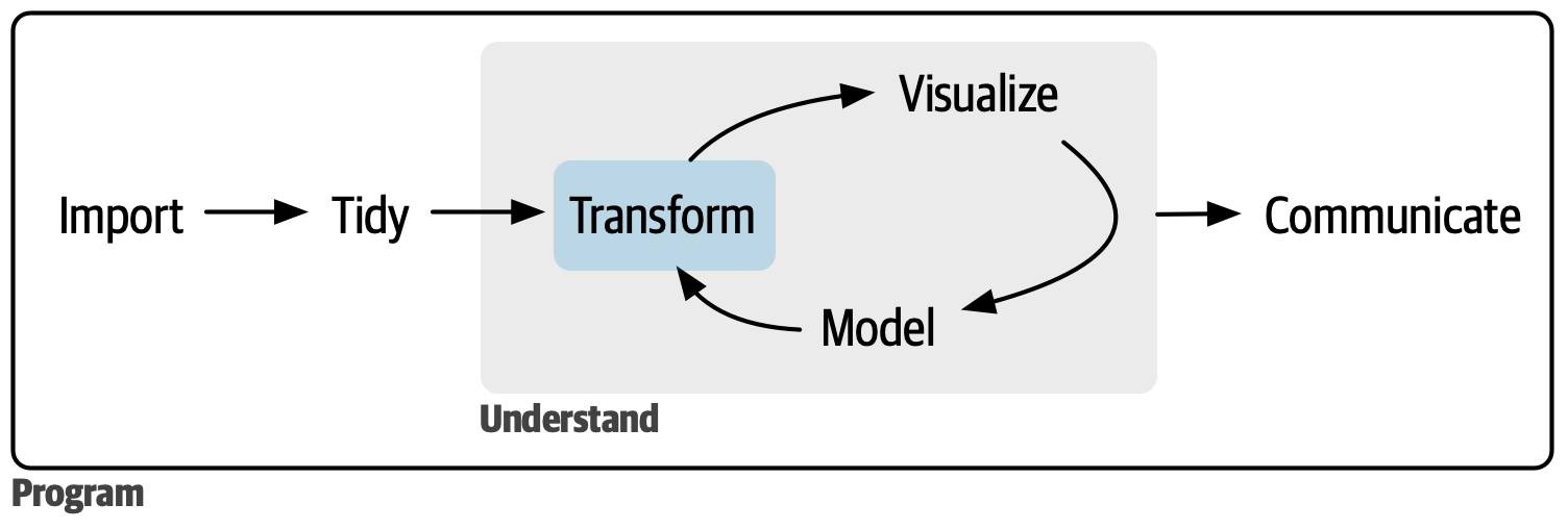
- For more information see the Transform chapter in the R4DS book https://r4ds.hadley.nz/transform.html
Goals
Setup
Logical vectors
Introduction
In this chapter, you’ll learn tools for working with logical vectors.
Logical vectors are the simplest type of vector because each element can only be one of three possible values:
TRUE,FALSE, andNA.It’s relatively rare to find logical vectors in your raw data, but you’ll create and manipulate them in the course of almost every analysis.
Introduction
We’ll begin by discussing the most common way of creating logical vectors: with numeric comparisons.
Then you’ll learn about how you can use Boolean algebra to combine different logical vectors, as well as some useful summaries.
We’ll finish off with
if_else()andcase_when(), two useful functions for making conditional changes powered by logical vectors.
Comparisons
A very common way to create a logical vector is via a numeric comparison with <, <=, >, >=, !=, and ==. So far, we’ve mostly created logical variables transiently within filter() — they are computed, used, and then thrown away. For example, the following filter finds all daytime departures that arrive roughly on time:
Comparisons
It’s useful to know that this is a shortcut and you can explicitly create the underlying logical variables with mutate():
Comparisons
This is particularly useful for more complicated logic because naming the intermediate steps makes it easier to both read your code and check that each step has been computed correctly.
All up, the initial filter is equivalent to:
flights |>
  mutate(
    daytime = dep_time > 600 & dep_time < 2000,
    approx_ontime = abs(arr_delay) < 20,
  ) |>
  filter(daytime & approx_ontime)
# A tibble: 172,286 × 21
year month day dep_time sched_dep_time dep_delay arr_time sched_arr_time
<int> <int> <int> <int> <int> <dbl> <int> <int>
1 2013 1 1 601 600 1 844 850
2 2013 1 1 602 610 -8 812 820
3 2013 1 1 602 605 -3 821 805
4 2013 1 1 606 610 -4 858 910
5 2013 1 1 606 610 -4 837 845
6 2013 1 1 607 607 0 858 915
7 2013 1 1 611 600 11 945 931
8 2013 1 1 613 610 3 925 921
9 2013 1 1 615 615 0 833 842
10 2013 1 1 622 630 -8 1017 1014
# ℹ 172,276 more rows
# ℹ 13 more variables: arr_delay <dbl>, carrier <chr>, flight <int>,
# tailnum <chr>, origin <chr>, dest <chr>, air_time <dbl>, distance <dbl>,
# hour <dbl>, minute <dbl>, time_hour <dttm>, daytime <lgl>,
# approx_ontime <lgl>Floating point comparison
Beware of using == with numbers. For example, it looks like this vector contains the numbers 1 and 2:
Floating point comparison
But if you test them for equality, you get FALSE:
What’s going on?
Computers store numbers with a fixed number of decimal places so there’s no way to exactly represent 1/49 or sqrt(2) and subsequent computations will be very slightly off. We can see the exact values by calling print() with the digits argument:
What’s going on?
You can see why R defaults to rounding these numbers; they really are very close to what you expect.
Now that you’ve seen why == is failing, what can you do about it?
Solution
One option is to use dplyr::near() which ignores small differences:
Missing values
Missing values represent the unknown so they are “contagious”: almost any operation involving an unknown value will also be unknown:
The most confusing result is this one:
Missing values
It’s easiest to understand why this is true if we artificially supply a little more context:
Missing values
So if you want to find all flights where dep_time is missing, the following code doesn’t work because dep_time == NA will yield NA for every single row, and filter() automatically drops missing values:
# A tibble: 0 × 19
# ℹ 19 variables: year <int>, month <int>, day <int>, dep_time <int>,
#   sched_dep_time <int>, dep_delay <dbl>, arr_time <int>,
#   sched_arr_time <int>, arr_delay <dbl>, carrier <chr>, flight <int>,
#   tailnum <chr>, origin <chr>, dest <chr>, air_time <dbl>, distance <dbl>,
#   hour <dbl>, minute <dbl>, time_hour <dttm>
Missing values
Instead we’ll need a new tool: is.na().
is.na(x) works with any type of vector and returns TRUE for missing values and FALSE for everything else:
Missing values
We can use is.na() to find all the rows with a missing dep_time:
# A tibble: 8,255 × 19
    year month   day dep_time sched_dep_time dep_delay arr_time sched_arr_time
   <int> <int> <int>    <int>          <int>     <dbl>    <int>          <int>
 1  2013     1     1       NA           1630        NA       NA           1815
 2  2013     1     1       NA           1935        NA       NA           2240
 3  2013     1     1       NA           1500        NA       NA           1825
 4  2013     1     1       NA            600        NA       NA            901
 5  2013     1     2       NA           1540        NA       NA           1747
 6  2013     1     2       NA           1620        NA       NA           1746
 7  2013     1     2       NA           1355        NA       NA           1459
 8  2013     1     2       NA           1420        NA       NA           1644
 9  2013     1     2       NA           1321        NA       NA           1536
10  2013     1     2       NA           1545        NA       NA           1910
# ℹ 8,245 more rows
# ℹ 11 more variables: arr_delay <dbl>, carrier <chr>, flight <int>,
#   tailnum <chr>, origin <chr>, dest <chr>, air_time <dbl>, distance <dbl>,
#   hour <dbl>, minute <dbl>, time_hour <dttm>
Missing values
is.na() can also be useful in arrange(). arrange() usually puts all the missing values at the end but you can override this default by first sorting by is.na():
# A tibble: 842 × 19
    year month   day dep_time sched_dep_time dep_delay arr_time sched_arr_time
   <int> <int> <int>    <int>          <int>     <dbl>    <int>          <int>
 1  2013     1     1      517            515         2      830            819
 2  2013     1     1      533            529         4      850            830
 3  2013     1     1      542            540         2      923            850
 4  2013     1     1      544            545        -1     1004           1022
 5  2013     1     1      554            600        -6      812            837
 6  2013     1     1      554            558        -4      740            728
 7  2013     1     1      555            600        -5      913            854
 8  2013     1     1      557            600        -3      709            723
 9  2013     1     1      557            600        -3      838            846
10  2013     1     1      558            600        -2      753            745
# ℹ 832 more rows
# ℹ 11 more variables: arr_delay <dbl>, carrier <chr>, flight <int>,
#   tailnum <chr>, origin <chr>, dest <chr>, air_time <dbl>, distance <dbl>,
#   hour <dbl>, minute <dbl>, time_hour <dttm>
Missing values
is.na() can also be useful in arrange(). arrange() usually puts all the missing values at the end but you can override this default by first sorting by is.na():
# A tibble: 842 × 19
    year month   day dep_time sched_dep_time dep_delay arr_time sched_arr_time
   <int> <int> <int>    <int>          <int>     <dbl>    <int>          <int>
 1  2013     1     1       NA           1630        NA       NA           1815
 2  2013     1     1       NA           1935        NA       NA           2240
 3  2013     1     1       NA           1500        NA       NA           1825
 4  2013     1     1       NA            600        NA       NA            901
 5  2013     1     1      517            515         2      830            819
 6  2013     1     1      533            529         4      850            830
 7  2013     1     1      542            540         2      923            850
 8  2013     1     1      544            545        -1     1004           1022
 9  2013     1     1      554            600        -6      812            837
10  2013     1     1      554            558        -4      740            728
# ℹ 832 more rows
# ℹ 11 more variables: arr_delay <dbl>, carrier <chr>, flight <int>,
#   tailnum <chr>, origin <chr>, dest <chr>, air_time <dbl>, distance <dbl>,
#   hour <dbl>, minute <dbl>, time_hour <dttm>
Missing values
The rules for missing values in Boolean algebra are a little tricky to explain because they seem inconsistent at first glance:
Missing values
To understand what’s going on, think about NA | TRUE (NA or TRUE).
A missing value in a logical vector means that the value could either be TRUE or FALSE.
TRUE | TRUEandFALSE | TRUEare bothTRUEbecause at least one of them isTRUE.NA | TRUEmust also beTRUEbecauseNAcan either beTRUEorFALSE.However,
NA | FALSEisNAbecause we don’t know ifNAisTRUEorFALSE.Similar reasoning applies with
NA & FALSE.
Order of operations
Note that the order of operations doesn’t work like English. Take the following code that finds all flights that departed in November or December:
Order of operations
You might be tempted to write it like you’d say in English: “Find all flights that departed in November or December.”:
# A tibble: 336,776 × 19
    year month   day dep_time sched_dep_time dep_delay arr_time sched_arr_time
   <int> <int> <int>    <int>          <int>     <dbl>    <int>          <int>
 1  2013     1     1      517            515         2      830            819
 2  2013     1     1      533            529         4      850            830
 3  2013     1     1      542            540         2      923            850
 4  2013     1     1      544            545        -1     1004           1022
 5  2013     1     1      554            600        -6      812            837
 6  2013     1     1      554            558        -4      740            728
 7  2013     1     1      555            600        -5      913            854
 8  2013     1     1      557            600        -3      709            723
 9  2013     1     1      557            600        -3      838            846
10  2013     1     1      558            600        -2      753            745
# ℹ 336,766 more rows
# ℹ 11 more variables: arr_delay <dbl>, carrier <chr>, flight <int>,
#   tailnum <chr>, origin <chr>, dest <chr>, air_time <dbl>, distance <dbl>,
#   hour <dbl>, minute <dbl>, time_hour <dttm>
Order of operations
This code doesn’t error but it also doesn’t seem to have worked.
What’s going on?
Here, R first evaluates
month == 11creating a logical vector, which we callnov.
Order of operations
It computes nov | 12. When you use a number with a logical operator it converts everything apart from 0 to TRUE, so this is equivalent to nov | TRUE which will always be TRUE, so every row will be selected:
# A tibble: 336,776 × 3
   month nov   final
   <int> <lgl> <lgl>
 1     1 FALSE TRUE
 2     1 FALSE TRUE
 3     1 FALSE TRUE
 4     1 FALSE TRUE
 5     1 FALSE TRUE
 6     1 FALSE TRUE
 7     1 FALSE TRUE
 8     1 FALSE TRUE
 9     1 FALSE TRUE
10     1 FALSE TRUE
# ℹ 336,766 more rows
%in%
An easy way to avoid the problem of getting your ==s and |s in the right order is to use %in%. x %in% y returns a logical vector the same length as x that is TRUE whenever a value in x is anywhere in y .
%in%
So to find all flights in November and December we could write:
%in%
Note that %in% obeys different rules for NA to ==, as NA %in% NA is TRUE.
%in%
This can make for a useful shortcut:
# A tibble: 8,803 × 19
    year month   day dep_time sched_dep_time dep_delay arr_time sched_arr_time
   <int> <int> <int>    <int>          <int>     <dbl>    <int>          <int>
 1  2013     1     1      800            800         0     1022           1014
 2  2013     1     1      800            810       -10      949            955
 3  2013     1     1       NA           1630        NA       NA           1815
 4  2013     1     1       NA           1935        NA       NA           2240
 5  2013     1     1       NA           1500        NA       NA           1825
 6  2013     1     1       NA            600        NA       NA            901
 7  2013     1     2      800            810       -10     1102           1116
 8  2013     1     2       NA           1540        NA       NA           1747
 9  2013     1     2       NA           1620        NA       NA           1746
10  2013     1     2       NA           1355        NA       NA           1459
# ℹ 8,793 more rows
# ℹ 11 more variables: arr_delay <dbl>, carrier <chr>, flight <int>,
#   tailnum <chr>, origin <chr>, dest <chr>, air_time <dbl>, distance <dbl>,
#   hour <dbl>, minute <dbl>, time_hour <dttm>
Summaries
The following sections describe some useful techniques for summarizing logical vectors. As well as functions that only work specifically with logical vectors, you can also use functions that work with numeric vectors.
Logical summaries
There are two main logical summaries:
any(x)is the equivalent of|; it’ll returnTRUEif there are anyTRUE’s inx.all(x)is equivalent of&; it’ll returnTRUEonly if all values ofxareTRUE’s.
Like all summary functions, they’ll return NA if there are any missing values present
You can make the missing values go away with na.rm = TRUE.
Logical summaries
For example, we could use all() and any() to find out if every flight was delayed on departure by at most an hour or if any flights were delayed on arrival by five hours or more. And using group_by() allows us to do that by day:
flights |>
  group_by(year, month, day) |>
  summarize(
    all_delayed = all(dep_delay <= 60, na.rm = TRUE),
    any_long_delay = any(arr_delay >= 300, na.rm = TRUE),
    .groups = "drop"
  )
# A tibble: 365 × 5
year month day all_delayed any_long_delay
<int> <int> <int> <lgl> <lgl>
1 2013 1 1 FALSE TRUE
2 2013 1 2 FALSE TRUE
3 2013 1 3 FALSE FALSE
4 2013 1 4 FALSE FALSE
5 2013 1 5 FALSE TRUE
6 2013 1 6 FALSE FALSE
7 2013 1 7 FALSE TRUE
8 2013 1 8 FALSE FALSE
9 2013 1 9 FALSE TRUE
10 2013 1 10 FALSE TRUE
# ℹ 355 more rowsLogical summaries
In most cases, however, any() and all() are a little too crude, and it would be nice to be able to get a little more detail about how many values are TRUE or FALSE.
That leads us to the numeric summaries.
Numeric summaries of logical vectors
When you use a logical vector in a numeric context, TRUE becomes 1 and FALSE becomes 0.
This makes sum() and mean() very useful
sum(x)gives the number ofTRUEsmean(x)gives the proportion ofTRUEs (becausemean()is justsum()divided bylength()).
Numeric summaries of logical vectors
That, for example, allows us to see the proportion of flights that were delayed on departure by at most an hour and the number of flights that were delayed on arrival by five hours or more:
flights |>
  group_by(year, month, day) |>
  summarize(
    proportion_delayed = mean(dep_delay <= 60, na.rm = TRUE),
    count_long_delay = sum(arr_delay >= 300, na.rm = TRUE),
    .groups = "drop"
  )
# A tibble: 365 × 5
year month day proportion_delayed count_long_delay
<int> <int> <int> <dbl> <int>
1 2013 1 1 0.939 3
2 2013 1 2 0.914 3
3 2013 1 3 0.941 0
4 2013 1 4 0.953 0
5 2013 1 5 0.964 1
6 2013 1 6 0.959 0
7 2013 1 7 0.956 1
8 2013 1 8 0.975 0
9 2013 1 9 0.986 1
10 2013 1 10 0.977 2
# ℹ 355 more rowsLogical subsetting
You can use a logical vector to filter a single variable to a subset of interest.
This makes use of the base [] (pronounced subset) operator
Logical subsetting example
Imagine we wanted to look at the average delay just for flights that were actually delayed. One way to do so would be to first filter the flights and then calculate the average delay:
flights |>
  filter(arr_delay > 0) |>
  group_by(year, month, day) |>
  summarize(
    behind = mean(arr_delay),
    n = n(),
    .groups = "drop"
  )
# A tibble: 365 × 5
year month day behind n
<int> <int> <int> <dbl> <int>
1 2013 1 1 32.5 461
2 2013 1 2 32.0 535
3 2013 1 3 27.7 460
4 2013 1 4 28.3 297
5 2013 1 5 22.6 238
6 2013 1 6 24.4 381
7 2013 1 7 27.8 243
8 2013 1 8 20.8 275
9 2013 1 9 25.6 287
10 2013 1 10 27.3 220
# ℹ 355 more rowsLogical subsetting example
This works, but what if we wanted to also compute the average delay for flights that arrived early?
We’d need to perform a separate filter step,
Next, join the two data frames together.
Instead you could use [ to perform an inline filtering: arr_delay[arr_delay > 0] will yield only the positive arrival delays.
Logical subsetting example
This leads to:
flights |>
  group_by(year, month, day) |>
  summarize(
    behind = mean(arr_delay[arr_delay > 0], na.rm = TRUE),
    ahead = mean(arr_delay[arr_delay < 0], na.rm = TRUE),
    n = n(),
    .groups = "drop"
  )
# A tibble: 365 × 6
year month day behind ahead n
<int> <int> <int> <dbl> <dbl> <int>
1 2013 1 1 32.5 -12.5 842
2 2013 1 2 32.0 -14.3 943
3 2013 1 3 27.7 -18.2 914
4 2013 1 4 28.3 -17.0 915
5 2013 1 5 22.6 -14.0 720
6 2013 1 6 24.4 -13.6 832
7 2013 1 7 27.8 -17.0 933
8 2013 1 8 20.8 -14.3 899
9 2013 1 9 25.6 -13.0 902
10 2013 1 10 27.3 -16.4 932
# ℹ 355 more rowsAlso note the difference in the group size: in the first chunk n() gives the number of delayed flights per day; in the second, n() gives the total number of flights.
Conditional transformations
One of the most powerful features of logical vectors are their use for conditional transformations, i.e. doing one thing for condition x, and something different for condition y. There are two important tools for this: if_else() and case_when().
if_else()
If you want to use one value when a condition is TRUE and another value when it’s FALSE, you can use dplyr::if_else().
You’ll always use the first three argument of if_else().
The first argument,
condition, is a logical vector,The second,
true, gives the output when the condition is true,The third,
false, gives the output if the condition is false.
if_else()
Let’s begin with a simple example of labeling a numeric vector as either “+ve” (positive) or “-ve” (negative):
if_else()
There’s an optional fourth argument, missing which will be used if the input is NA:
if_else()
You can also use vectors for the true and false arguments. For example, this allows us to create a minimal implementation of abs():
case_when()
Syntax to recreate our nested if_else() as follows:
case_when()
Use .default if you want to create a “default”/catch all value:
case_when()
Use .default if you want to create a “default”/catch all value:
case_when()
And note that if multiple conditions match, only the first will be used:
case_when() example
flights |>
  mutate(
    status = case_when(
      is.na(arr_delay)      ~ "cancelled",
      arr_delay < -30       ~ "very early",
      arr_delay < -15       ~ "early",
      abs(arr_delay) <= 15  ~ "on time",
      arr_delay < 60        ~ "late",
      arr_delay < Inf       ~ "very late",
    ),
    .keep = "used"
  )
# A tibble: 336,776 × 2
arr_delay status
<dbl> <chr>
1 11 on time
2 20 late
3 33 late
4 -18 early
5 -25 early
6 12 on time
7 19 late
8 -14 on time
9 -8 on time
10 8 on time
# ℹ 336,766 more rowsBe wary when writing this sort of complex case_when() statement; my first two attempts used a mix of < and > and I kept accidentally creating overlapping conditions.
Compatible types
Note that both if_else() and case_when() require compatible types in the output. If they’re not compatible, you’ll see errors like this:
Compatible types
Overall, relatively few types are compatible, because automatically converting one type of vector to another is a common source of errors. Here are the most important cases that are compatible:
- Numeric and logical vectors are compatible.
- Strings and factors are compatible, because you can think of a factor as a string with a restricted set of values.
- Dates and date-times are compatible because you can think of a date as a special case of date-time.
NA, which is technically a logical vector, is compatible with everything because every vector has some way of representing a missing value.