Data transformations

Lecture 9

2025-03-17

Warm up

Setup

── Attaching core tidyverse packages ──────────────────────── tidyverse 2.0.0 ──
✔ dplyr     1.1.4     ✔ readr     2.1.5
✔ forcats   1.0.0     ✔ stringr   1.5.1
✔ ggplot2   3.5.1     ✔ tibble    3.2.1
✔ lubridate 1.9.4     ✔ tidyr     1.3.1
✔ purrr     1.0.4     
── Conflicts ────────────────────────────────────────── tidyverse_conflicts() ──
✖ dplyr::filter() masks stats::filter()
✖ dplyr::lag()    masks stats::lag()
ℹ Use the conflicted package (<http://conflicted.r-lib.org/>) to force all conflicts to become errors

Introduction

Prerequisites

• Numeric vectors are the backbone of data science
• But we still need the tidyverse because we’ll use these base R functions inside of tidyverse functions like mutate() and filter().

library(tidyverse)
library(nycflights13)

Making numbers

In most cases, you’ll get numbers already recorded in one of R’s numeric types:

• integer

• double.

In some cases, however, you’ll encounter them as strings, possibly because you’ve created them by pivoting from column headers or because something has gone wrong in your data import process.

Parsing numbers

readr provides two useful functions for parsing strings into numbers: parse_double() and parse_number(). Use parse_double() when you have numbers that have been written as strings:

x <- c("1.2", "5.6", "1e3")
parse_double(x)

[1]    1.2    5.6 1000.0

Use parse_number() when the string contains non-numeric text that you want to ignore. This is particularly useful for currency data and percentages:

x <- c("$1,234", "USD 3,513", "59%")
parse_number(x)

[1] 1234 3513   59

Counts

The dplyr::count() is great for quick exploration and checks during analysis:

flights |> count(dest)

# A tibble: 105 × 2
   dest      n
   <chr> <int>
 1 ABQ     254
 2 ACK     265
 3 ALB     439
 4 ANC       8
 5 ATL   17215
 6 AUS    2439
 7 AVL     275
 8 BDL     443
 9 BGR     375
10 BHM     297
# ℹ 95 more rows

Counts

If you want to see the most common values, add sort = TRUE:

flights |> count(dest, sort = TRUE)

# A tibble: 105 × 2
   dest      n
   <chr> <int>
 1 ORD   17283
 2 ATL   17215
 3 LAX   16174
 4 BOS   15508
 5 MCO   14082
 6 CLT   14064
 7 SFO   13331
 8 FLL   12055
 9 MIA   11728
10 DCA    9705
# ℹ 95 more rows

If you want to see all the values:

• |> View()

• |> print(n = Inf).

Counts alternative

Same computation “by hand” with group_by(), summarize() and n().

flights |> 
  group_by(dest) |> 
  summarize(
    n = n(),
    delay = mean(arr_delay, na.rm = TRUE)
  )

# A tibble: 105 × 3
   dest      n delay
   <chr> <int> <dbl>
 1 ABQ     254  4.38
 2 ACK     265  4.85
 3 ALB     439 14.4 
 4 ANC       8 -2.5 
 5 ATL   17215 11.3 
 6 AUS    2439  6.02
 7 AVL     275  8.00
 8 BDL     443  7.05
 9 BGR     375  8.03
10 BHM     297 16.9 
# ℹ 95 more rows

Count distinct

There are a couple of variants of n() and count() that you might find useful:

• n_distinct(x) counts the number of distinct (unique) values of one or more variables. For example, we could figure out which destinations are served by the most carriers:

  flights |> 
    group_by(dest) |> 
    summarize(carriers = n_distinct(carrier)) |> 
    arrange(desc(carriers))

  # A tibble: 105 × 2
     dest  carriers
     <chr>    <int>
   1 ATL          7
   2 BOS          7
   3 CLT          7
   4 ORD          7
   5 TPA          7
   6 AUS          6
   7 DCA          6
   8 DTW          6
   9 IAD          6
  10 MSP          6
  # ℹ 95 more rows

Weighted count

• A weighted count is a sum. For example you could “count” the number of miles each plane flew:

  flights |> 
    group_by(tailnum) |> 
    summarize(miles = sum(distance))

  # A tibble: 4,044 × 2
     tailnum  miles
     <chr>    <dbl>
   1 D942DN    3418
   2 N0EGMQ  250866
   3 N10156  115966
   4 N102UW   25722
   5 N103US   24619
   6 N104UW   25157
   7 N10575  150194
   8 N105UW   23618
   9 N107US   21677
  10 N108UW   32070
  # ℹ 4,034 more rows

Weighted count

Weighted counts are a common problem so count() has a wt argument that does the same thing:

```{r}
#| results: false
flights |> count(tailnum, wt = distance)
```

Counts missing

• You can count missing values by combining sum() and is.na(). In the flights dataset this represents flights that are cancelled:

  flights |> 
    group_by(dest) |> 
    summarize(n_cancelled = sum(is.na(dep_time))) 

  # A tibble: 105 × 2
     dest  n_cancelled
     <chr>       <int>
   1 ABQ             0
   2 ACK             0
   3 ALB            20
   4 ANC             0
   5 ATL           317
   6 AUS            21
   7 AVL            12
   8 BDL            31
   9 BGR            15
  10 BHM            25
  # ℹ 95 more rows

Numeric transformations

Transformation functions work well with mutate() because their output is the same length as the input.

Minimum and maximum

The arithmetic functions work with pairs of variables (or columns). Two closely related functions are pmin() and pmax(), which when given two or more variables will return the smallest or largest value in each row:

df <- tribble(
  ~x, ~y,
  1,  3,
  5,  2,
  7, NA,
)

df |> 
  mutate(
    min = pmin(x, y, na.rm = TRUE),
    max = pmax(x, y, na.rm = TRUE)
  )

# A tibble: 3 × 4
      x     y   min   max
  <dbl> <dbl> <dbl> <dbl>
1     1     3     1     3
2     5     2     2     5
3     7    NA     7     7

Minimum and maximum

Note that these are different to the summary functions min() and max() which take multiple observations and return a single value. You can tell that you’ve used the wrong form when all the minimums and all the maximums have the same value:

df |> 
  mutate(
    min = min(x, y, na.rm = TRUE),
    max = max(x, y, na.rm = TRUE)
  )

# A tibble: 3 × 4
      x     y   min   max
  <dbl> <dbl> <dbl> <dbl>
1     1     3     1     7
2     5     2     1     7
3     7    NA     1     7

Modular arithmetic

Modular arithmetic is the technical name for the type of math you did before you learned about decimal places, i.e. division that yields a whole number and a remainder. In R, %/% does integer division and %% computes the remainder:

1:10 %/% 3

 [1] 0 0 1 1 1 2 2 2 3 3

1:10 %% 3

 [1] 1 2 0 1 2 0 1 2 0 1

Modular arithmetic

Modular arithmetic is handy for the flights dataset, because we can use it to unpack the sched_dep_time variable into hour and minute:

flights |> 
  mutate(
    hour = sched_dep_time %/% 100,
    minute = sched_dep_time %% 100,
    .keep = "used"
  )

# A tibble: 336,776 × 3
   sched_dep_time  hour minute
            <int> <dbl>  <dbl>
 1            515     5     15
 2            529     5     29
 3            540     5     40
 4            545     5     45
 5            600     6      0
 6            558     5     58
 7            600     6      0
 8            600     6      0
 9            600     6      0
10            600     6      0
# ℹ 336,766 more rows

Modular arithmetic

We can combine that with the mean(is.na(x)) trick from ?@sec-logical-summaries to see how the proportion of cancelled flights varies over the course of the day. The results are shown in Figure 1.

flights |> 
  group_by(hour = sched_dep_time %/% 100) |> 
  summarize(prop_cancelled = mean(is.na(dep_time)), n = n()) |> 
  filter(hour > 1) |> 
  ggplot(aes(x = hour, y = prop_cancelled)) +
  geom_line(color = "grey50") + 
  geom_point(aes(size = n))

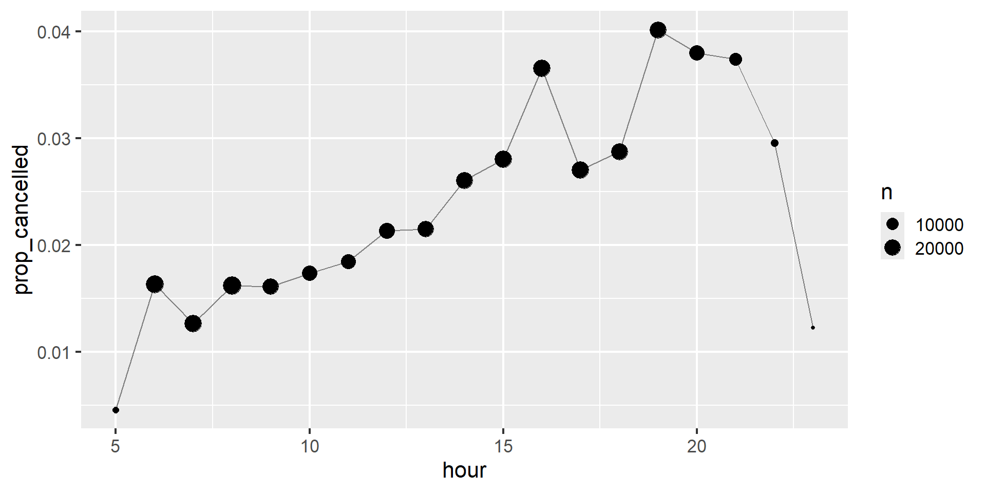
Figure 1: A line plot with scheduled departure hour on the x-axis, and proportion of cancelled flights on the y-axis. Cancellations seem to accumulate over the course of the day until 8pm, very late flights are much less likely to be cancelled.

Logarithms

Three logarithms

In R, you have a choice of three logarithms:

• log() (the natural log, base e),

• log2() (base 2),

• log10() (base 10).

Logarithm recommendation

We recommend using log2() or log10():

• log2() is easy to interpret because a difference of 1 on the log scale corresponds to doubling on the original scale and a difference of -1 corresponds to halving;

• log10() is easy to back-transform because (e.g.) 3 is 10^3 = 1000.

The inverse of log() is exp(); to compute the inverse of log2() or log10() you’ll need to use 2^ or 10^.

Rounding

Use round(x) to round a number to the nearest integer:

round(123.456)

[1] 123

Rounding digits

You can control the precision of the rounding with the second argument, digits. round(x, digits) rounds to the nearest 10^-n so digits = 2 will round to the nearest 0.01. This definition is useful because it implies round(x, -3) will round to the nearest thousand, which indeed it does:

round(123.456, 2)  # two digits

[1] 123.46

round(123.456, 1)  # one digit

[1] 123.5

round(123.456, -1) # round to nearest ten

[1] 120

round(123.456, -2) # round to nearest hundred

[1] 100

Rounding digits - weirdness

There’s one weirdness with round() that seems surprising at first glance:

round(c(1.5, 2.5))

[1] 2 2

round() uses what’s known as “round half to even” or Banker’s rounding: if a number is half way between two integers, it will be rounded to the even integer. This is a good strategy because it keeps the rounding unbiased: half of all 0.5s are rounded up, and half are rounded down.

Rounding digits - floor/ceiling

round() is paired with floor() which always rounds down and ceiling() which always rounds up:

x <- 123.456

floor(x)

[1] 123

ceiling(x)

[1] 124

Cutting numbers into ranges

Use cut()¹ to break up (aka bin) a numeric vector into discrete buckets:

x <- c(1, 2, 5, 10, 15, 20)
x

[1]  1  2  5 10 15 20

cut(x, breaks = c(0, 5, 10, 15, 20))

[1] (0,5]   (0,5]   (0,5]   (5,10]  (10,15] (15,20]
Levels: (0,5] (5,10] (10,15] (15,20]

1. ggplot2 provides some helpers for common cases in cut_interval(), cut_number(), and cut_width(). ggplot2 is an admittedly weird place for these functions to live, but they are useful as part of histogram computation and were written before any other parts of the tidyverse existed.

Cutting numbers into ranges

The breaks don’t need to be evenly spaced:

cut(x, breaks = c(0, 5, 10, 100))

[1] (0,5]    (0,5]    (0,5]    (5,10]   (10,100] (10,100]
Levels: (0,5] (5,10] (10,100]

Cutting numbers into ranges

You can optionally supply your own labels. Note that there should be one less labels than breaks.

cut(x, 
  breaks = c(0, 5, 10, 15, 20), 
  labels = c("sm", "md", "lg", "xl")
)

[1] sm sm sm md lg xl
Levels: sm md lg xl

Cutting numbers into ranges

Any values outside of the range of the breaks will become NA:

y <- c(NA, -10, 5, 10, 30)
cut(y, breaks = c(0, 5, 10, 15, 20))

[1] <NA>   <NA>   (0,5]  (5,10] <NA>  
Levels: (0,5] (5,10] (10,15] (15,20]

See the documentation for other useful arguments like right and include.lowest, which control if the intervals are [a, b) or (a, b] and if the lowest interval should be [a, b].

Cumulative and rolling aggregates

Base R provides cumsum(), cumprod(), cummin(), cummax() for running, or cumulative, sums, products, mins and maxes. dplyr provides cummean() for cumulative means. Cumulative sums tend to come up the most in practice:

x <- 1:10
x

 [1]  1  2  3  4  5  6  7  8  9 10

cumprod(x)

 [1]       1       2       6      24     120     720    5040   40320  362880
[10] 3628800

If you need more complex rolling or sliding aggregates, try the slider package.

General transformations

The following sections describe some general transformations which are often used with numeric vectors, but can be applied to all other column types.

Ranks

dplyr provides a number of ranking functions inspired by SQL, but you should always start with dplyr::min_rank(). It uses the typical method for dealing with ties, e.g., 1st, 2nd, 2nd, 4th.

x <- c(1, 3, 2, 2, 4, 20, 15, NA)
min_rank(x)

[1]  1  4  2  2  5  7  6 NA

Ranks

Note that the smallest values get the lowest ranks; use desc(x) to give the largest values the smallest ranks:

min_rank(desc(x))

[1]  7  4  5  5  3  1  2 NA

Ranks alternatives

If min_rank() doesn’t do what you need, look at the variants dplyr::row_number(), dplyr::dense_rank(), dplyr::percent_rank(), and dplyr::cume_dist(). See the documentation for details.

df <- tibble(x = x)
df |> 
  mutate(
    row_number = row_number(x),
    dense_rank = dense_rank(x),
    percent_rank = percent_rank(x),
    cume_dist = cume_dist(x)
  )

# A tibble: 8 × 5
      x row_number dense_rank percent_rank cume_dist
  <dbl>      <int>      <int>        <dbl>     <dbl>
1     1          1          1        0         0.143
2     3          4          3        0.5       0.571
3     2          2          2        0.167     0.429
4     2          3          2        0.167     0.429
5     4          5          4        0.667     0.714
6    20          7          6        1         1    
7    15          6          5        0.833     0.857
8    NA         NA         NA       NA        NA    

Offsets

dplyr::lead() and dplyr::lag() allow you to refer to the values just before or just after the “current” value. They return a vector of the same length as the input, padded with NAs at the start or end:

x <- c(2, 5, 11, 11, 19, 35)
lag(x)

[1] NA  2  5 11 11 19

lead(x)

[1]  5 11 11 19 35 NA

Offsets - lag

• x - lag(x) gives you the difference between the current and previous value.

  x - lag(x)

  [1] NA  3  6  0  8 16

• x == lag(x) tells you when the current value changes.

  x == lag(x)

  [1]    NA FALSE FALSE  TRUE FALSE FALSE

You can lead or lag by more than one position by using the second argument, n.

Consecutive identifiers

Sometimes you want to start a new group every time some event occurs. For example, when you’re looking at website data, it’s common to want to break up events into sessions, where you begin a new session after a gap of more than x minutes since the last activity. For example, imagine you have the times when someone visited a website:

events <- tibble(
  time = c(0, 1, 2, 3, 5, 10, 12, 15, 17, 19, 20, 27, 28, 30)
)

Consecutive identifiers

And you’ve computed the time between each event, and figured out if there’s a gap that’s big enough to qualify:

events <- events |> 
  mutate(
    diff = time - lag(time, default = first(time)),
    has_gap = diff >= 5
  )
events

# A tibble: 14 × 3
    time  diff has_gap
   <dbl> <dbl> <lgl>  
 1     0     0 FALSE  
 2     1     1 FALSE  
 3     2     1 FALSE  
 4     3     1 FALSE  
 5     5     2 FALSE  
 6    10     5 TRUE   
 7    12     2 FALSE  
 8    15     3 FALSE  
 9    17     2 FALSE  
10    19     2 FALSE  
11    20     1 FALSE  
12    27     7 TRUE   
13    28     1 FALSE  
14    30     2 FALSE  

Consecutive identifiers

But how do we go from that logical vector to something that we can group_by()? cumsum(), from Section 5.11, comes to the rescue as gap, i.e. has_gap is TRUE, will increment group by one (?@sec-numeric-summaries-of-logicals):

events |> mutate(
  group = cumsum(has_gap)
)

# A tibble: 14 × 4
    time  diff has_gap group
   <dbl> <dbl> <lgl>   <int>
 1     0     0 FALSE       0
 2     1     1 FALSE       0
 3     2     1 FALSE       0
 4     3     1 FALSE       0
 5     5     2 FALSE       0
 6    10     5 TRUE        1
 7    12     2 FALSE       1
 8    15     3 FALSE       1
 9    17     2 FALSE       1
10    19     2 FALSE       1
11    20     1 FALSE       1
12    27     7 TRUE        2
13    28     1 FALSE       2
14    30     2 FALSE       2

Consecutive identifiers

Another approach for creating grouping variables is consecutive_id(), which starts a new group every time one of its arguments changes. For example, inspired by this stackoverflow question, imagine you have a data frame with a bunch of repeated values:

df <- tibble(
  x = c("a", "a", "a", "b", "c", "c", "d", "e", "a", "a", "b", "b"),
  y = c(1, 2, 3, 2, 4, 1, 3, 9, 4, 8, 10, 199)
)

Consecutive identifiers

If you want to keep the first row from each repeated x, you could use group_by(), consecutive_id(), and slice_head():

df |> 
  group_by(id = consecutive_id(x)) |> 
  slice_head(n = 1)

# A tibble: 7 × 3
# Groups:   id [7]
  x         y    id
  <chr> <dbl> <int>
1 a         1     1
2 b         2     2
3 c         4     3
4 d         3     4
5 e         9     5
6 a         4     6
7 b        10     7

Numeric summaries

Just using the counts, means, and sums that we’ve introduced already can get you a long way, but R provides many other useful summary functions. Here is a selection that you might find useful.

Center

• Function mean()
• Function median()

Minimum, maximum, and quantiles

• min() and max() will give you the largest and smallest values.
• Another powerful tool is quantile() which is a generalization of the median:
  • quantile(x, 0.25) will find the value of x that is greater than 25% of the values,
  • quantile(x, 0.5) is equivalent to the median,
  • quantile(x, 0.95) will find the value that’s greater than 95% of the values.

Minimum, maximum, and quantiles

For the flights data, you might want to look at the 95% quantile of delays rather than the maximum, because it will ignore the 5% of most delayed flights which can be quite extreme.

flights |>
  group_by(year, month, day) |>
  summarize(
    max = max(dep_delay, na.rm = TRUE),
    q95 = quantile(dep_delay, 0.95, na.rm = TRUE),
    .groups = "drop"
  )

# A tibble: 365 × 5
    year month   day   max   q95
   <int> <int> <int> <dbl> <dbl>
 1  2013     1     1   853  70.1
 2  2013     1     2   379  85  
 3  2013     1     3   291  68  
 4  2013     1     4   288  60  
 5  2013     1     5   327  41  
 6  2013     1     6   202  51  
 7  2013     1     7   366  51.6
 8  2013     1     8   188  35.3
 9  2013     1     9  1301  27.2
10  2013     1    10  1126  31  
# ℹ 355 more rows

Variation

Two commonly used summaries are

• the standard deviation sd(x),

• the inter-quartile range, IQR().

Positions

There’s one final type of summary that’s useful for numeric vectors, but also works with every other type of value: extracting a value at a specific position:

• first(x),

• last(x), and

• nth(x, n).

Positions

For example, we can find the first, fifth and last departure for each day:

flights |> 
  group_by(year, month, day) |> 
  summarize(
    first_dep = first(dep_time, na_rm = TRUE), 
    fifth_dep = nth(dep_time, 5, na_rm = TRUE),
    last_dep = last(dep_time, na_rm = TRUE)
  )

`summarise()` has grouped output by 'year', 'month'. You can override using the
`.groups` argument.

# A tibble: 365 × 6
# Groups:   year, month [12]
    year month   day first_dep fifth_dep last_dep
   <int> <int> <int>     <int>     <int>    <int>
 1  2013     1     1       517       554     2356
 2  2013     1     2        42       535     2354
 3  2013     1     3        32       520     2349
 4  2013     1     4        25       531     2358
 5  2013     1     5        14       534     2357
 6  2013     1     6        16       555     2355
 7  2013     1     7        49       536     2359
 8  2013     1     8       454       544     2351
 9  2013     1     9         2       524     2252
10  2013     1    10         3       530     2320
# ℹ 355 more rows

NB: Because dplyr functions use _ to separate components of function and arguments names, these functions use na_rm instead of na.rm.

With mutate()

As the names suggest, the summary functions are typically paired with summarize(). However, because of the recycling rules we discussed in ?@sec-recycling they can also be usefully paired with mutate(), particularly when you want do some sort of group standardization. For example:

• x / sum(x) calculates the proportion of a total.
• (x - mean(x)) / sd(x) computes a Z-score (standardized to mean 0 and sd 1).
• (x - min(x)) / (max(x) - min(x)) standardizes to range [0, 1].
• x / first(x) computes an index based on the first observation.